Minkowski Asteroids
We have two convex polygons P and Q each moving at constant velocities Vp and Vq. At some point in time they may pass through one another. We would like to find the point in time at which the area of their intersection is at a maximum. Here is a simple visualization, where the yellow area represents the intersection and the arrow heads represents the velocity of the polygons.

Let’s first look at the problem of testing whether two polygons intersect. The simplest way to do it is to check if any edges of one polygon intersect any edges of the other. For this we need a line segment intersection algorithm. We can check if two line segments A - B and C - D intersect if the signed area of the triangle A, B, C is different from the signed area of the triangle A, B, D and similarly for C, D, A and C, D, B. It’s simple and runs in O(N^2). Here’s the code:
import numpy as np

def area(A, B, C):
     return np.linalg.norm(np.cross(B - A, B - C)) * 0.5

def intersect(A, B, C, D):
    return area(A, B, C) != area(A, B, D) and area(C, D, A) != area(C, D, B)

def polygons_intersect(P, Q):
    n = len(P)
    m = len(P)
    for i in xrange(n):
        for j in xrange(m):
            if intersect(P[i], P[(i+1)%n], Q[j], Q[(j+1)%m]):
                return True
    return False
Aside: #
There is a another way to do this using something called the hyperplane separation theorem. Rather than explaining it I’ll plot an example of how it works in two dimensions, which I think is more helpful. Take each edge of the polygons in questions and extend them outwards in the direction of their normals. In the plots below the dotted lines represent normals and the solid lines, the extensions of and edges of one of the polygons. Let’s call extensions of the edges “barriers”. Now consider projecting both shapes onto any of the barriers. This would turn them into line segments on the barriers. In the case of intersection these segments would overlap on all the barriers. Look at this plot and confirm that projecting the shapes in the center onto any barrier would yield a solid line segment, not two.

This is different in the case where there is no intersection. In this case there is at least one barrier where the projection of the shapes do not for a solid line segment. In this example it’s the purple barrier and you can see that the normal to this barrier actually shows the separation of the shapes (purple dotted line). How do we check if the projection of the shapes on to the barrier intersect? We can project those segments again down onto something simple line a horizontal line and see if their endpoints overlap.

Armed with some fast polygon intersection algorithms we can go back to our original problem and try various points in time and check whether the polygons intersect. This is still not great because there is no guarantee that they will intersect and even then, what we are actually looking for is the range of times during which the shapes intersect so we can compute the maximum area of overlap.
Let’s try another approach. First let’s make a simplification and assume that one of the shapes is stationary and the other is moving relative to it. Let’s project each point on our moving polygon out in the direction of its velocity.
These rays may or may not intersect the other polygon. In this case we have four intersections. With each of the intersections we can compute a time based on the velocity of the polygon. We can sort these times and return the minimum and maximum as time range of overlap.
def overlap_range(P, Q, V):
    for x, y in zip(*Q.exterior.xy):

        # simulate a ray as a long line segment
        SCALE = 1e10
        segment_x = [ x, x + SCALE*V[0] ]
        segment_y = [ y, y + SCALE*V[1] ]
        line = [segment_x, segment_y]

        points = intersections(P, line)

        for point in points:
            ix, iy = point.x, point.y
            # time of intersection
            when = math.hypot(x-ix, y-iy) / math.hypot(V[0], V[1])

        intersection_times.append(when)

    intersection_times.sort()

    if len(intersection_time) == 0:
        print "polygons never overlap"
    elif len(intersection_time) == 1:
        print "polygons touch by don't overlap"

    return intersection_time[0], intersection_time[-1]
Here each point on the polygon creates a line segment and that is tested against each edge of the other polygon. So we’ve handled the issues of when the polygons don’t ever intersect but we can do even better with Minkowski geometry. We’ll use something called the Minkowski difference between two sets of points. In image processing it’s related to erosion. What this does is take one shape, mirror it about the origin and then compute the Minkowski sum of the mirrored shape and the other one. The Minkowski sum is related to dilation and for two sets of points P and Q is defined as all points p+q where p is in P and q is in Q.
Don’t worry two much about the definitions. Here is the key point to understand. We are looking to compute if the two polygons intersect. If they intersect there is a point in each polygon that is inside both of them. If so mirroring one polygon and computing the Minkowski sum polygon would create a polygon that contains the origin.
Here’s some code to compute the Minkowski difference between two polygons. Since both sets are convex we take the convex hull of the resulting polygon to create a new convex polygon.
def minkowski_difference(P, Q):

    R = []

    for i in xrange(len(P)):
        for j in xrange(len(Q)):
            R.append((P[i] - Q[j], P[i] - Q[j]))

    return convex_hull(R)
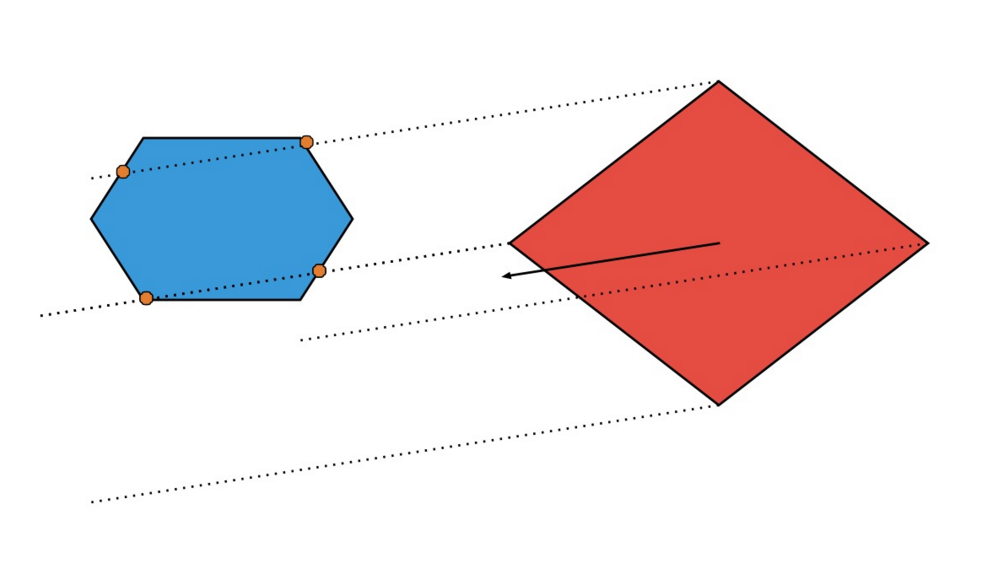
The convex hull is just the minimum sized convex polygon that encloses all the points. If you hammer a bunch of nails into a board and stretch an elastic band around all the the nails; the nails that touch the elastic band are the convex hull. It can be computed in O(N*log(N)) with a Graham Scan. Here’s a image showing two sets of points (red and blue) and their corresponding convex hulls. It also shows the intersection in yellow which is the convex hull of the points in both polygons and the intersection points. Seeing this go back and confirm the key point above that if the polygons intersect their Minkowski difference contains the origin.

Now instead of having two polygons we have one green polygon that is the Minkowski difference of the other two. In addition, from the definition of the Minkowski difference, we know that if the origin is inside this polygon the two comprising polygons intersect one another. This is a really important fact which let’s us compute collisions really fast and more importantly when the collision will happen. We can also compute the first and last points of intersection of these polygons using a single ray from the origin in the direction of the relative velocities of the polygons.
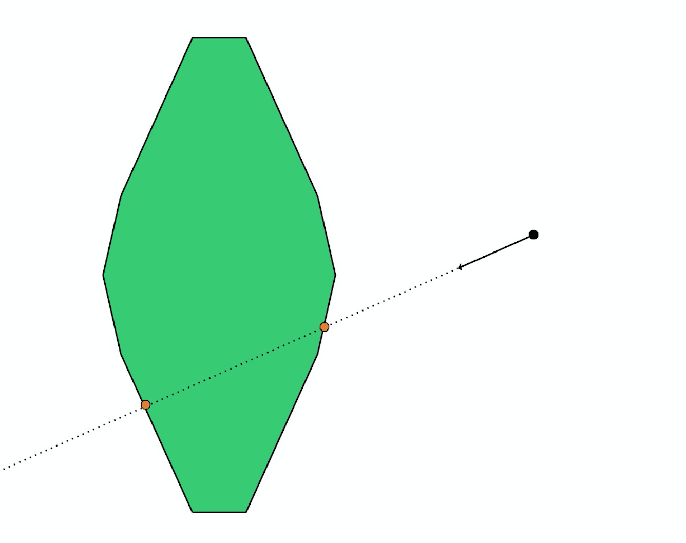
Here’s an illustration of what is happening in both normal and Minkowski space. You can see the blue and red polygons passing through one another. At the same time you can watch the green polygon representing the Minkowski difference between the red and blue polygon moving through the origin at the same time.

Once we’ve retrieved this range (the first and last intersection times) we can sample some points in that range and compute the overlap. The intersection of two convex polygons another convex polygon which is the convex hull of the intersections points and points that lie inside both polygons. Using our convex hull function and our intersection function we can compute this polygon and then use the Surveyor’s Algorithm to compute the area.
Finally putting all the pieces together we have an algorithm that takes the Minkowski difference of two polygons then computes the (generally) two points of intersection of the ray from the origin to the Minkowski difference polygon. Using the times of the two intersections we can compute the overlap of the two polygons as a function of time. Plotting the result we get this.

The final task remains to compute the maximum of this function. It seems that that the overlap is unimodal where the maximum is reached if one shape is entirely inside the other. Theres is proof in this paper . Since the function is unimodal we can use a ternary search to quickly compute the maximum in O(log N).
def findMax(objectiveFunc, lower, upper):

    if abs(upper - lower) < 1e-6:
        return (lower + upper)/2

    lowerThird = (2*lower + upper)/3
    upperThird = (lower + 2*upper)/3

    if objectiveFunc(lowerThird) < objectiveFunc(upperThird):
        return findMax(objectiveFunc, lowerThird, upper)
    else:
        return findMax(objectiveFunc, lower, upperThird)
Minkowski geometry extends to N dimensions and the principles stay the same - which can make it easier to do things like collision detection and response in 3 dimensions where the more simplistic methods don’t generalize well. This question was posed at the ICPC ACM World Finals.