Josef “Jeff” Sipek

Late last summer I decided to do a simple experiment—feed my server a PPS signal that wasn’t synchronized to any timescale. The idea was to give chrony a reference that is more stable than the crystal oscillator on the motherboard.

Hardware

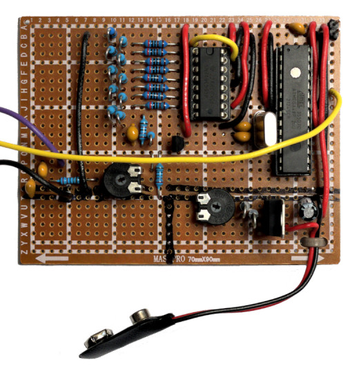
For this PPS experiment I decided to avoid all control loop/feedback complexity and just manually set the frequency to something close enough and let it drift—hence the unsynchronized. As a result, the circuit was quite simple:

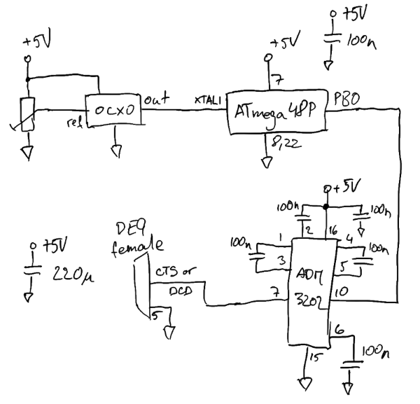
The OCXO was a $5 used part from eBay. It outputs a 10 MHz square wave and has a control voltage pin that lets you tweak the frequency a little bit. By playing with it, I determined that a 10mV control voltage change yielded about 0.1 Hz frequency change. The trimmer sets this reference voltage. To “calibrate” it, I connected it to a frequency counter and tweaked the trimmer until a frequency counter read exactly 10 MHz.

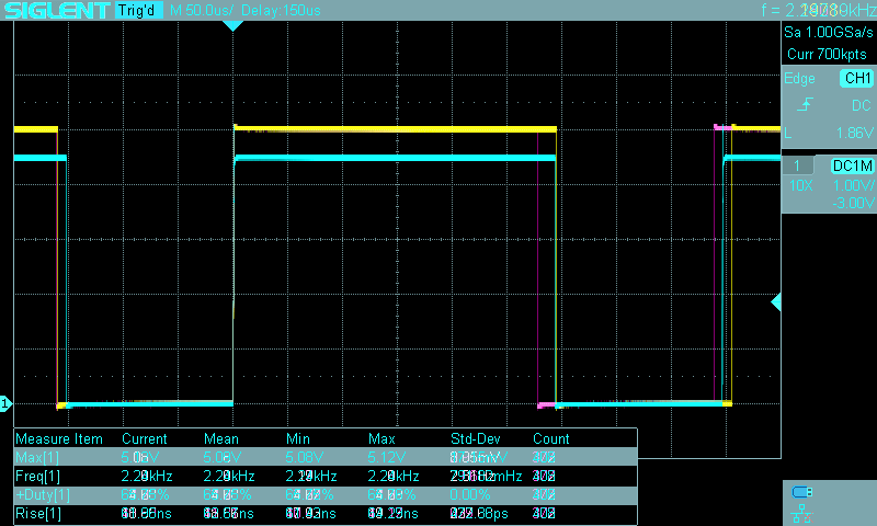
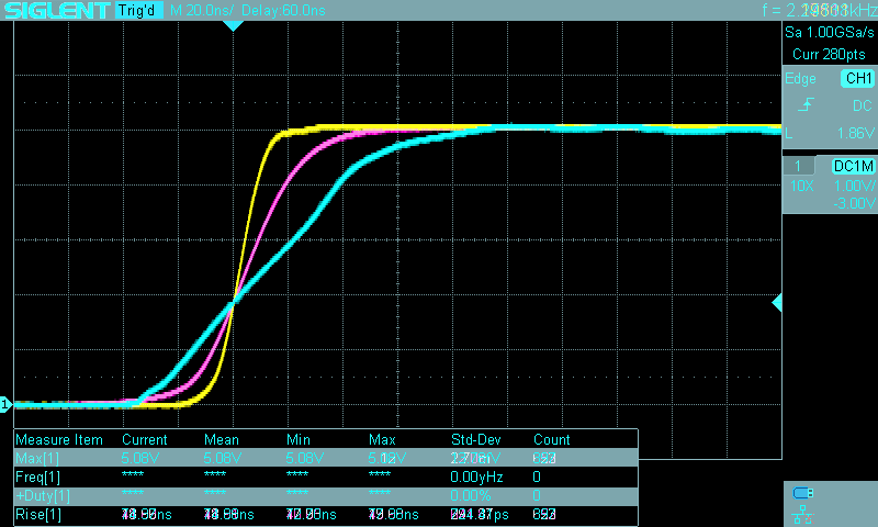
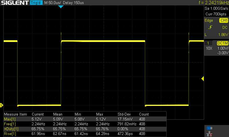
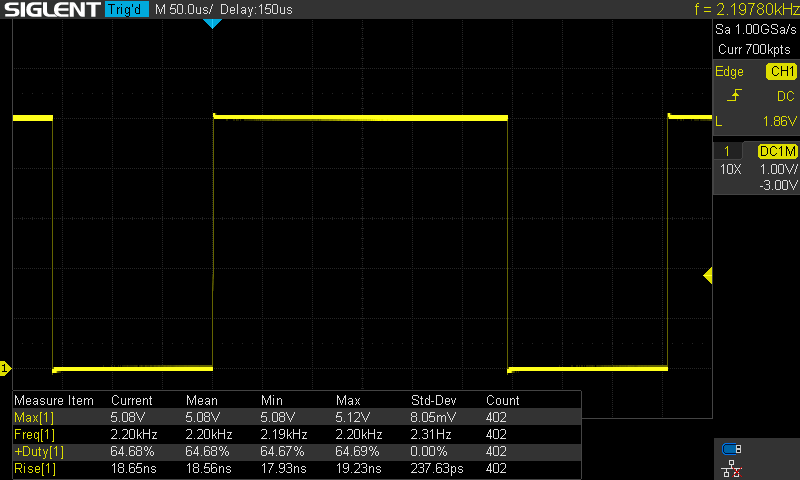
10 MHz is obviously way too fast for a PPS signal. The simplest way to turn it into a PPS signal is to use an 8-bit microcontroller. The ATmega48P’s design seems to have very deterministic timing (in other words it adds a negligible amount of jitter), so I used it at 10 MHz (fed directly from the OCXO) with a very simple assembly program to toggle an output pin on and off. The program kept an output pin high for exactly 2 million cycles, and low for 8 million cycles thereby creating a 20% duty cycle square wave at 1 Hz…perfect to use as a PPS. Since the jitter added by the microcontroller is measured in picoseconds it didn’t affect the overall performance in any meaningful way.

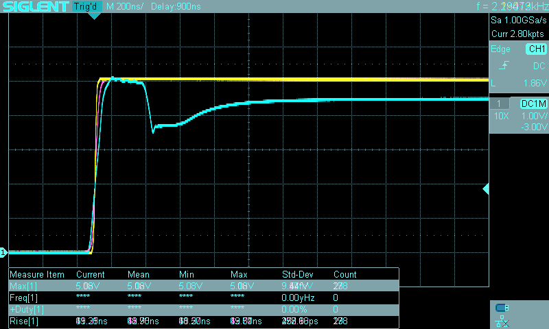
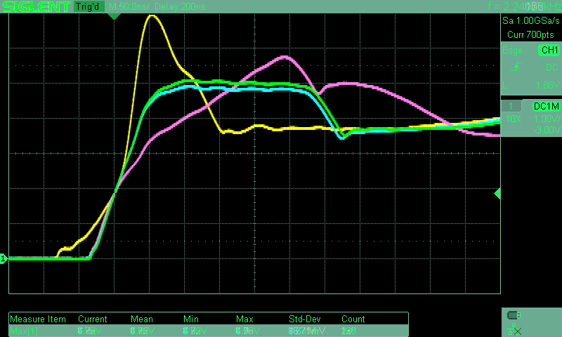
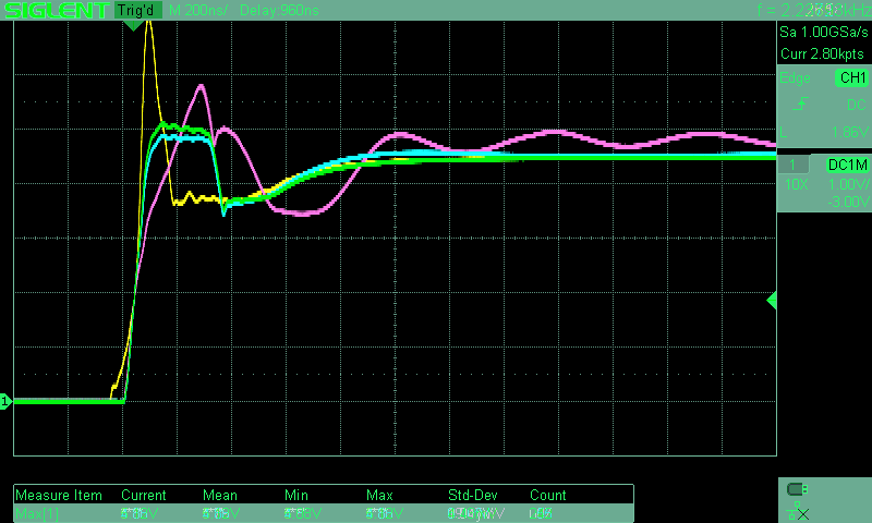
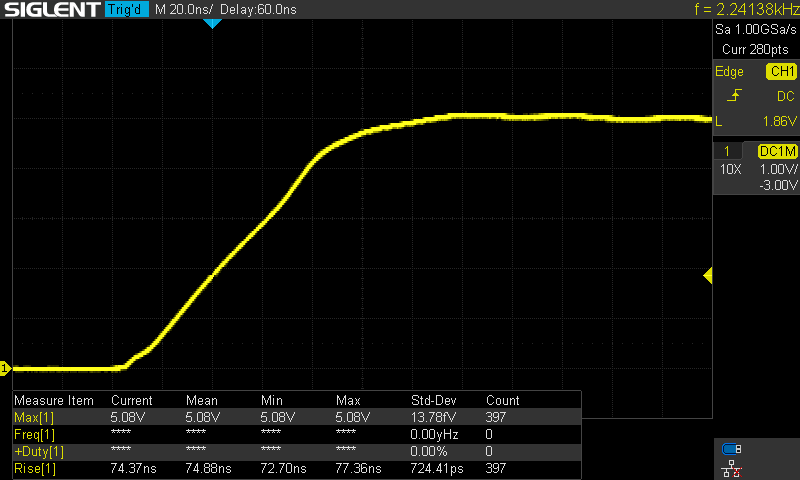
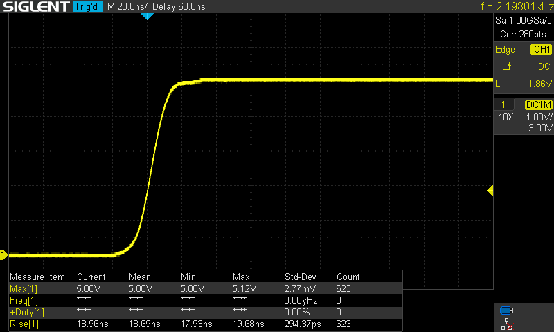
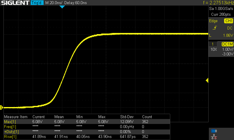
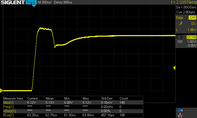
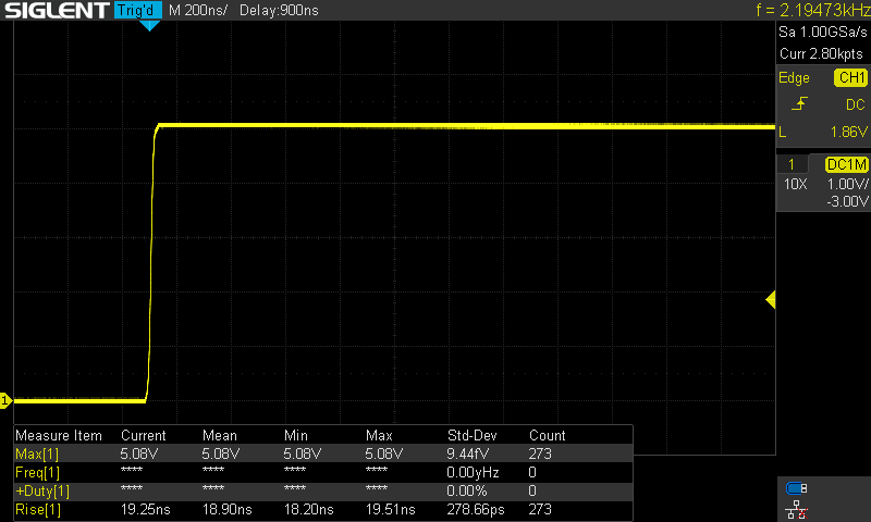
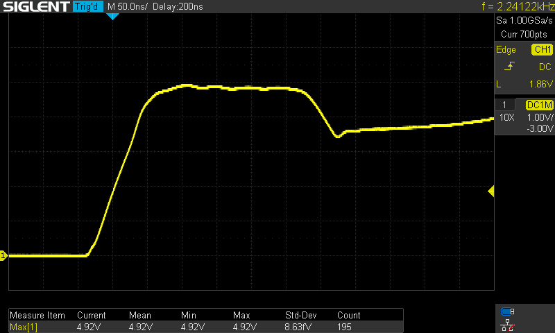
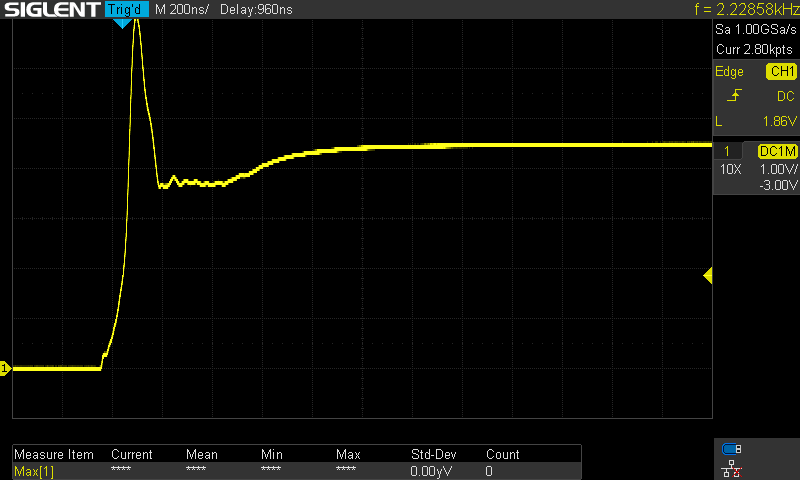
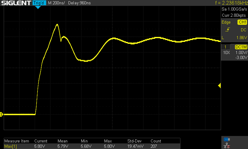
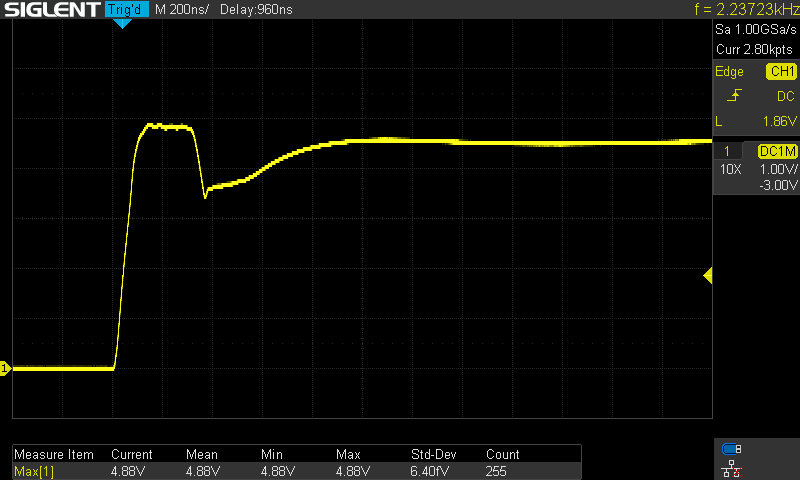
The ATmega48P likes to run at 5V and therefore its PPS output is +5V/0V, which isn’t compatible with a PC serial port. I happened to have an ADM3202 on hand so I used it to convert the 5V signal to an RS-232 compatible signal. I didn’t do as thorough of a check of its jitter characteristics, but I didn’t notice anything bad while testing the circuit before “deploying” it.

Finally, I connected the RS-232 compatible signal to the DCD pin (but CTS would have worked too).

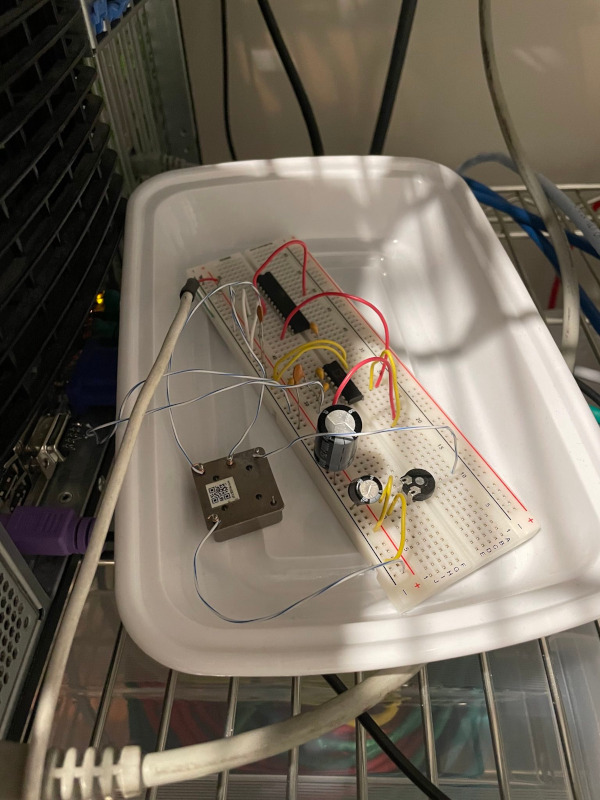
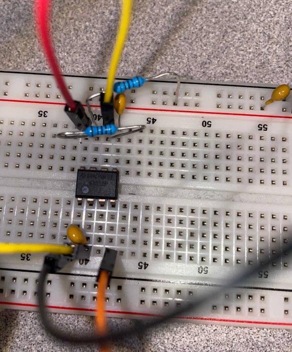
The whole circuit was constructed on a breadboard with the OCXO floating in the air on its wires. Power was supplied with an iPhone 5V USB power supply. Overall, it was a very quick and dirty construction to see how well it would work.

Software

My server runs FreeBSD with chrony as the NTP daemon. The configuration is really simple.

First, setting dev.uart.0.pps_mode to 2 informs the kernel that the PPS signal is on DCD (see uart(4)).

Second, we need to tell chrony that there is a local PPS on the port:

refclock PPS /dev/cuau0 local 

The local token is important. It tells chrony that the PPS is not synchronized to UTC. In other words, that the PPS can be used as a 1 Hz frequency source but not as a phase source.

Performance

I ran my server with this PPS refclock for about 50 days with chrony configured to log the time offset of each pulse and to apply filtering to every 16 pulses. (This removes some of the errors related to serial port interrupt handling not being instantaneous.) The following evaluation uses only these filtered samples as well as the logged data about the calculated system time error.

In addition to the PPS, chrony used several NTP servers from the internet (including the surprisingly good time.cloudflare.com) for the date and time-of-day information. This is a somewhat unfortunate situation when it comes to trying to figure out how good of an oscillator the OCXO is, as to make good conclusions about one oscillator one needs a better quality oscillator for the comparison. However, there are still a few things one can look at even when the (likely) best oscillator is the one being tested.

NTP Time Offset

The ultimate goal of a PPS source is to stabilize the system’s clock. Did the PPS source help? I think it is easy to answer that question by looking at the remaining time offset (column 11 in chrony’s tracking.log) over time.

This is a plot of 125 days that include the 50 days when I had the PPS circuit running. You can probably guess which 50 days. (The x-axis is time expressed as  Modified Julian Date, or MJD for short.)

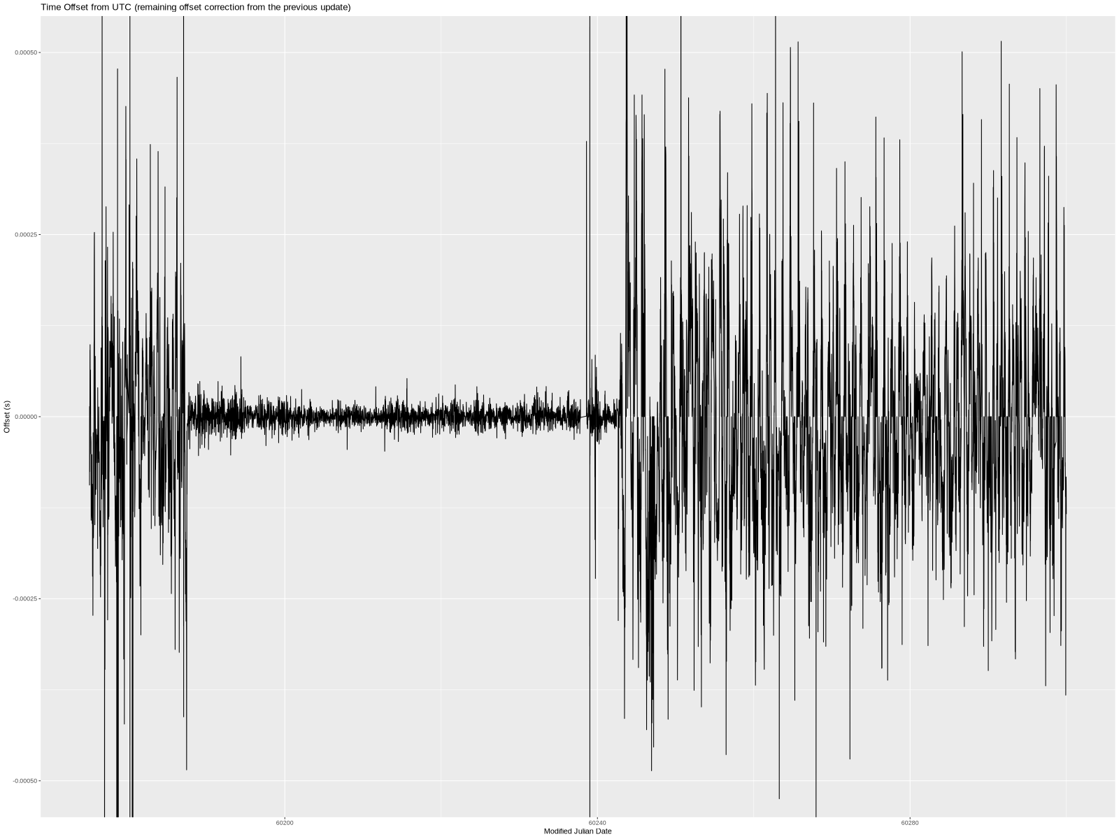
I don’t really have anything to say aside from—wow, what a difference!

For completeness, here’s a plot of the estimated local offset at the epoch (column 7 in tracking.log). My understanding of the difference between the two columns is fuzzy but regardless of which I go by, the improvement was significant.

Fitting a Polynomial Model

In addition to looking at the whole-system performance, I wanted to look at the PPS performance itself.

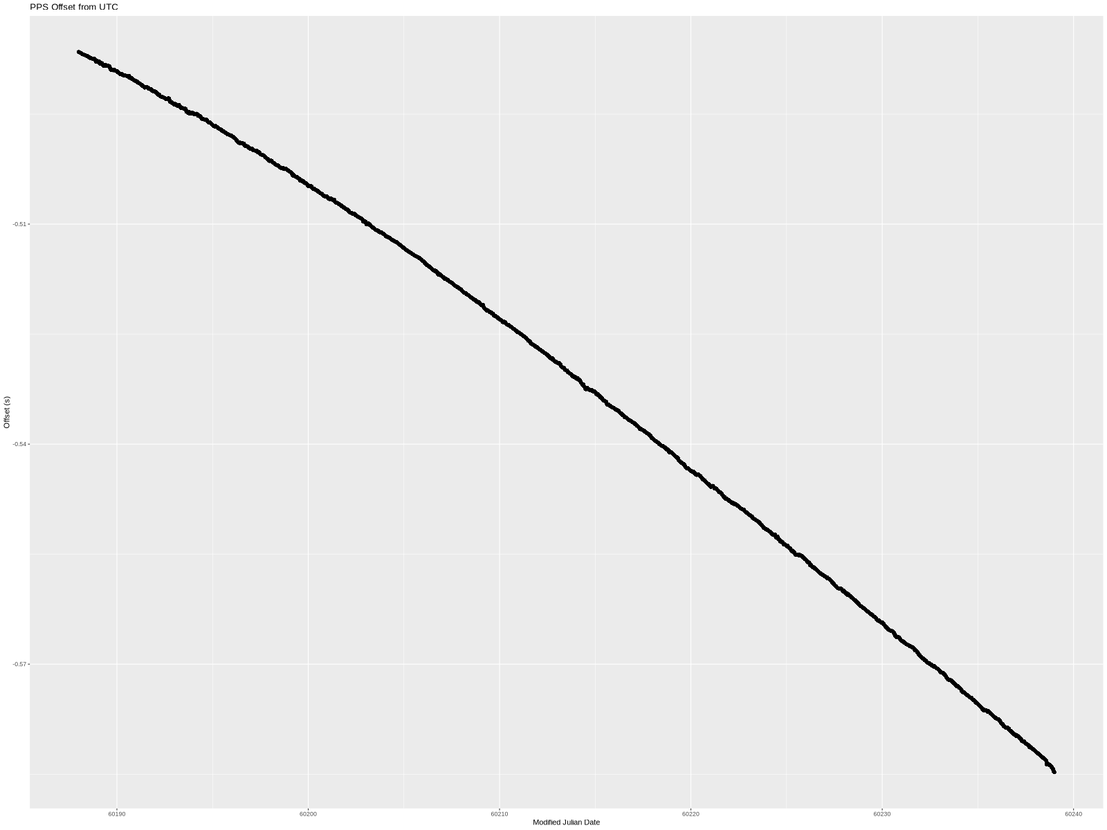
As before, the x-axis is MJD. The y-axis is the PPS offset as measured and logged by chrony—the 16-second filtered values.

The offset started at -486.5168ms. This is an arbitrary offset that simply shows that I started the PPS circuit about half a second off of UTC. Over the approximately 50 days, the offset grew to -584.7671ms.

This means that the OCXO frequency wasn’t exactly 10 MHz (and therefore the 1 PPS wasn’t actually at 1 Hz). Since there is a visible curve to the line, it isn’t a simple fixed frequency error but rather the frequency drifted during the experiment.

How much? I used  R’s lm function to fit simple polynomials to the collected data. I tried a few different polynomial degrees, but all of them were fitted the same way:

m <- lm(pps_offset ~ poly(time, poly_degree, raw=TRUE))
a <- as.numeric(m$coefficients[1])
b <- as.numeric(m$coefficients[2])
c <- as.numeric(m$coefficients[3])
d <- as.numeric(m$coefficients[4])

In all cases, these coefficients correspond to the 4 terms in $a+\mathrm{bt}+{\mathrm{ct}}^2+{\mathrm{dt}}^3$. For lower-degree polynomials, the missing coefficients are 0.

Note: Even though the plots show the x-axis in MJD, the calculations were done in seconds with the first data point at t=0 seconds.

Linear

The simplest model is a linear one. In other words, fitting a straight line through the data set. lm provided the following coefficients:

a=-0.480090626569894
b=-2.25787872135774e-08

That is an offset of -480.09ms and slope of -22.58ns/s (which is also -22.58 ppb frequency error).

Graphically, this is what the line looks like when overlayed on the measured data:

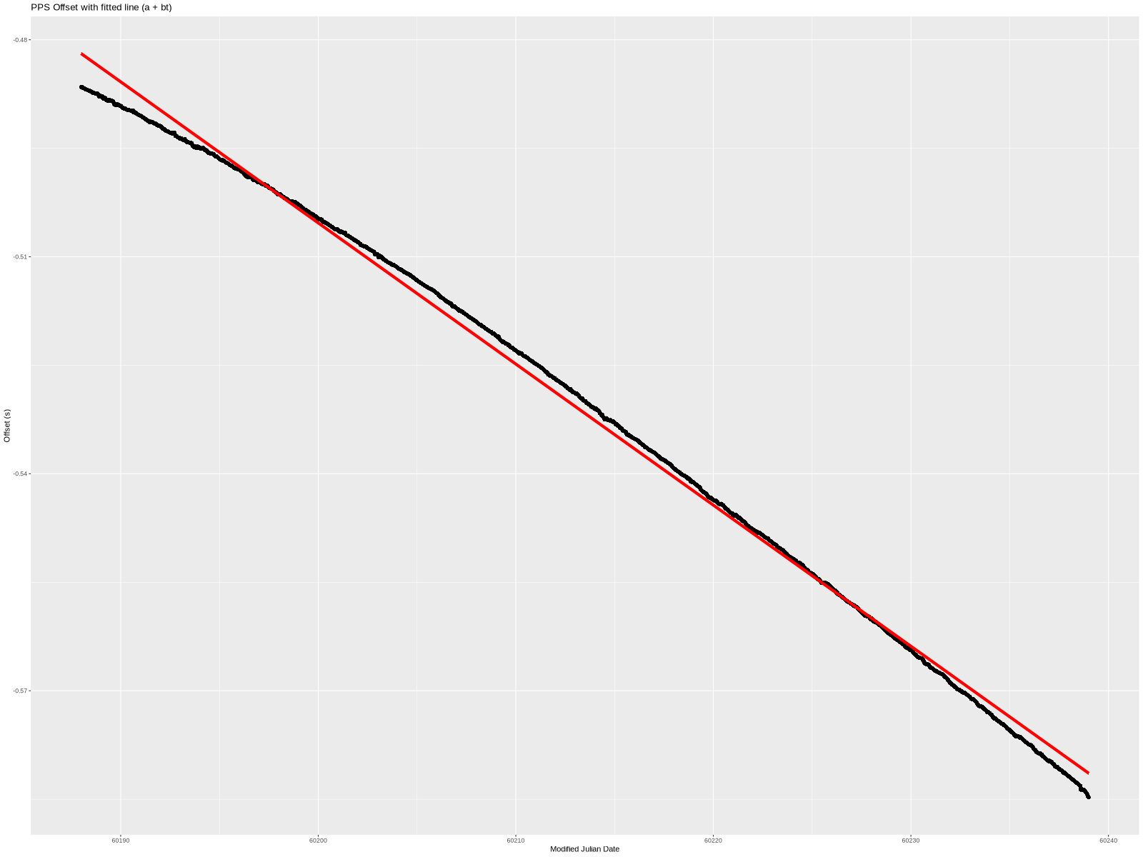
Not bad but also not great. Here is the difference between the two:

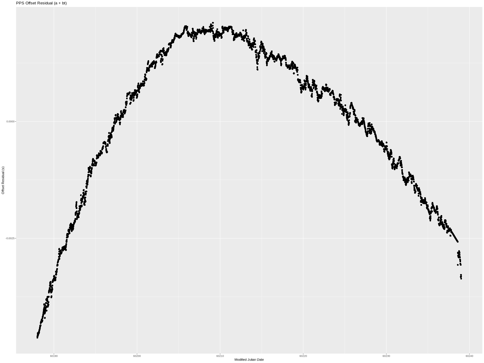
Put another way, this is the PPS offset from UTC if we correct for time offset (a) and a frequency error (b). The linear model clearly doesn’t handle the structure in the data completely. The residual is near low-single-digit milliseconds. We can do better, so let’s try to add another term.

Quadratic

lm produced these coefficients for a degree 2 polynomial:

a=-0.484064700277606
b=-1.75349684277379e-08
c=-1.10412099841665e-15

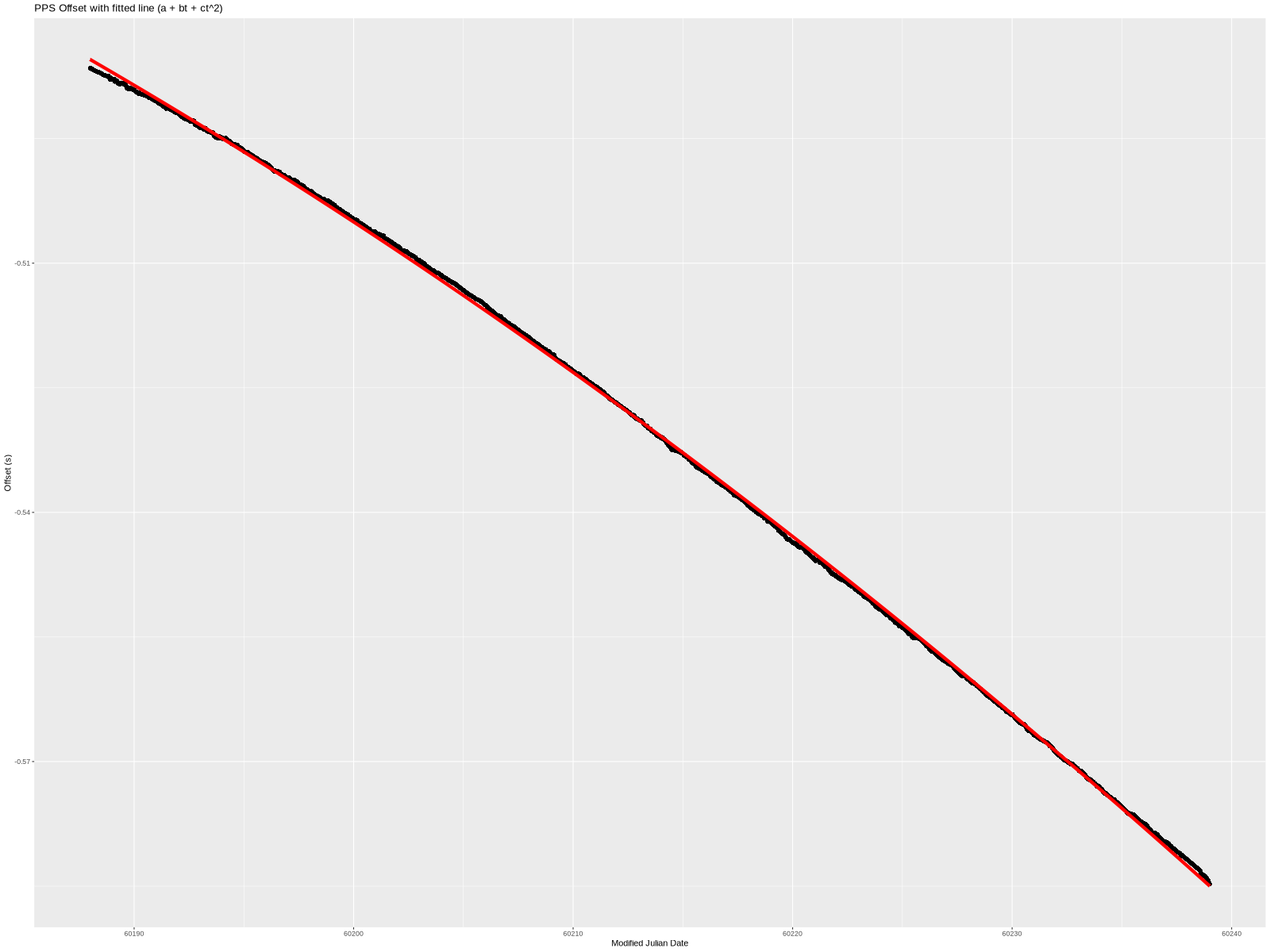
Visually, this fits the data much better. It’s a little wrong on the ends, but overall quite nice. Even the residual (below) is smaller—almost completely confined to less than 1 millisecond.

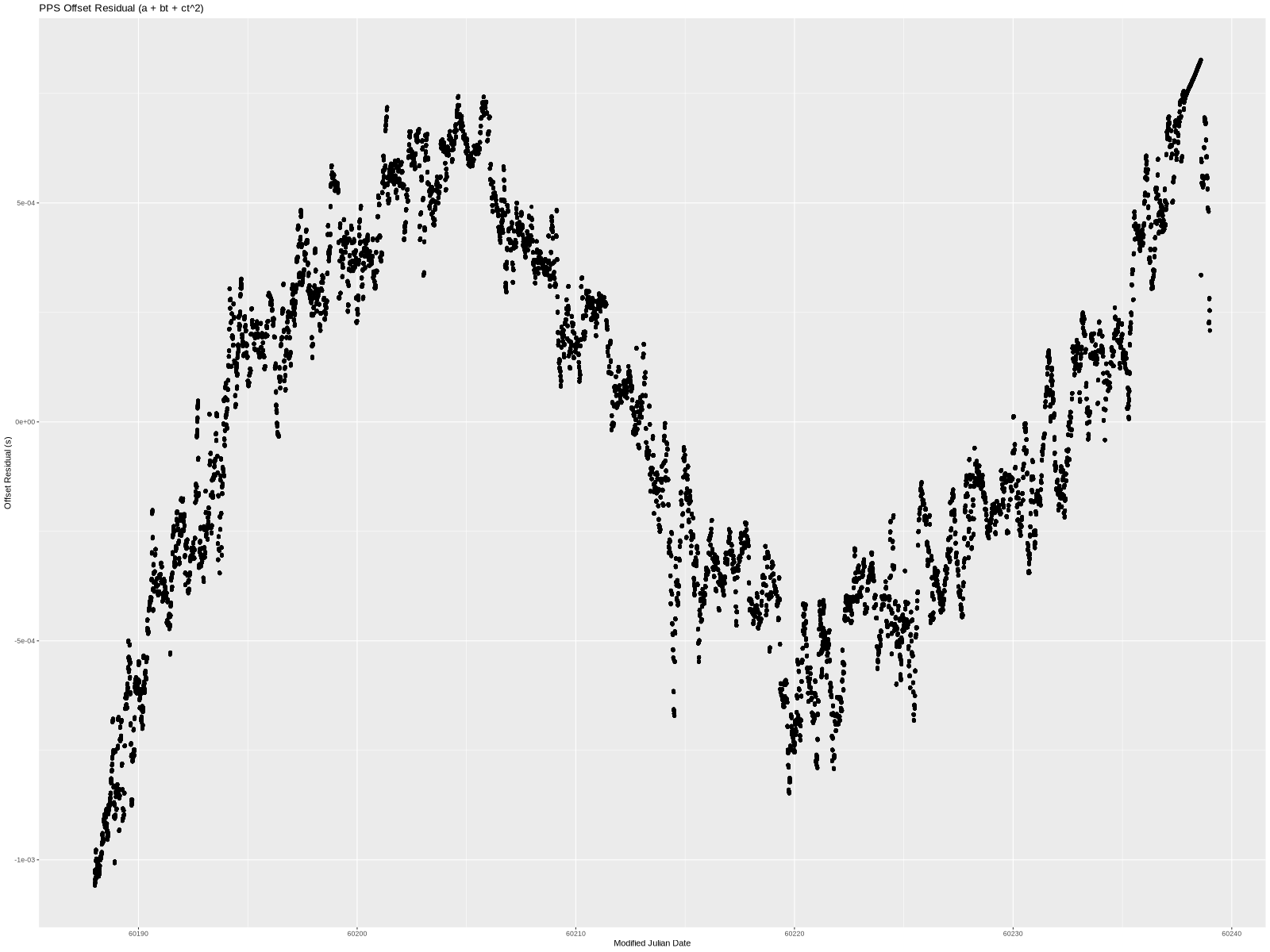
a is still time offset, b is still frequency error, and c is a time “acceleration” of sorts.

There is still very visible structure to the residual, so let’s add yet another term.

Cubic

As before, lm yielded the coefficients. This time they were:

a=-0.485357232306569
b=-1.44068934233748e-08
c=-2.78676248986831e-15
d=2.45563844387287e-22

That’s really close looking!

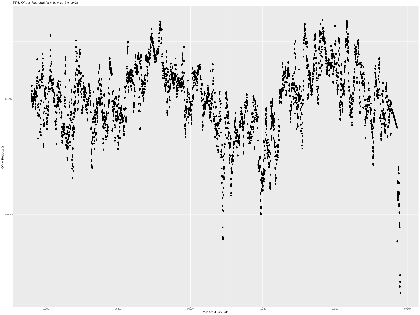
The residual still has a little bit of a wave to it, but almost all the data points are within 500 microseconds. I think that’s sufficiently close given just how much non-deterministic “stuff” (both hardware and software) there is between a serial port and an OS kernel’s interrupt handler on a modern server. (In theory, we could add additional terms forever until we completely eliminated the residual.)

So, we have a model of what happened to the PPS offset over time. Specifically, $a+\mathrm{bt}+{\mathrm{ct}}^2+{\mathrm{dt}}^3$ and the 4 constants. The offset (a of approximately -485ms) is easily explained—I started the PPS at the “wrong” time. The frequency error (b of approximately -14.4 ppb) can be explained as I didn’t tune the oscillator to exactly 10 MHz. (More accurately, I tuned it, unplugged it, moved it to my server, and plugged it back in. The slightly different environment could produce a few ppb error.)

What about the c and d terms? They account for a combination of a lot of things. Temperature is a big one. First of all, it is a home server and so it is subject to air-conditioner cycling on and off at a fairly long interval. This produces sizable swings in temperature, which in turn mess with the frequency. A server in a data center sees much less temperature variation, since the chillers keep the temperature essentially constant (at least compared to homes). Second, the oscillator was behind the server and I expect the temperature to slightly vary based on load.

One could no doubt do more analysis (and maybe at some point I will), but this post is already getting way too long.

Conclusion

One can go nuts trying to play with time and time synchronization. This is my first attempt at timekeeping-related circuitry, so I’m sure there are ways to improve the circuit or the analysis.

I think this experiment was a success. The system clock behavior improved beyond what’s needed for a general purpose server. Getting under 20 ppb error from a simple circuit on a breadboard with absolutely no control loop is great. I am, of course, already tinkering with various ideas that should improve the performance.

A recent upgrade of FreeBSD on my desktop resulted in just about every program (Firefox, KiCAD, but thankfully not urxvt) rendering various ligatures even for monospaced fonts. Needless to say, this is really annoying when looking at code, etc. Not having any better ideas, I asked on Mastodon if anyone knew how to turn this mis-feature off.

About an hour later, @monwarez@bsd.cafe suggested dropping the following XML in /usr/local/etc/fonts/conf.avail/29-local-noto-mono-fixup.conf and adding a symlink in ../conf.d to enable it:

<?xml version="1.0"?>
<!DOCTYPE fontconfig SYSTEM "urn:fontconfig:fonts.dtd">
<fontconfig>
	<description>Disable ligatures for monospaced fonts to avoid ff, fi, ffi, etc. becoming only one character wide</description>
	<match target="font">
		<test name="family" compare="eq">
			<string>Noto Sans Mono</string>
		</test>
		<edit name="fontfeatures" mode="append">
			<string>liga off</string>
			<string>dlig off</string>
		</edit>
	</match>
</fontconfig>

This solved my problem. Hopefully this will help others. if not, it’s a note-to-self for when I need to reapply this fixup :)

Yesterday, I saw KM1NDY’s blog post titled Scribbled Antenna Blueprints. I wasn’t going to comment…but here I am. :)

I thought I’d setup up a similar contraption (VHF instead of HF) to see what exactly happens. I have a 1 meter long RG-8X jumper with BNC connectors, a BNC T, and a NanoVNA with a 50Ω load calibration standard.

But first, let’s analyze the situation!

Imagine you have a transmitter/signal generator and you connect it to a dummy load. Assuming ideal components, absolutely nothing would get radiated. Now, imagine inserting an open stub between the two. In other words, the T has the following connections:

1. the generator
2. 50Ω load
3. frequency-dependant impedance

Let’s do trivial math! Let’s call the total load that the generator sees $Z_{\mathrm{total}}$ and the impedance provided by the stub $Z_{\mathrm{stub}}$. The generator side of the T is connected to the other ports in parallel. Therefore:

$Z_{\mathrm{total}}=\frac{50*Z_{\mathrm{stub}}}{50+Z_{\mathrm{stub}}}$

So, when would we get a 1:1 SWR? When the generator sees a 50Ω load. When will it see 50Ω? When $Z_{\mathrm{stub}}$ is very large; the extreme of which is when that side of the T is open.

If you are a ham, you may remember from when you were studying for the Amateur Extra exam that transmission line stubs can transform impedance. A 1/2 wave stub “copies” the impedance. A 1/4 wave stub “inverts” the impedance. For this “experiment” we need a high impedance. We can get that by either:

1. open 1/2 wave stub
2. shorted 1/4 wave stub

Since the “design” from the scribble called for an open, we’ll focus on the 1/2 wave open stub.

Now, back to the experiment. I have a 1 m long RG-8X which has a velocity factor of 0.78. So, let’s calculate the frequency for which it is a 1/2 wave—i.e., the frequency where the wavelength is 2 times the length of the coax:

$f=0.78*c/2m$

This equals 116.9 MHz. So, we should expect 1:1 SWR at 117-ish MHz. (The cable is approximately 1 m long and the connectors and the T add some length, so it should be a bit under 117.)

Oh look! 1.015:1 SWR at 110.5 MHz.

(Using 1.058 m in the calculation yields 110.5 MHz. I totally believe that between the T and the connectors there is close to 6 cm of extra (electrical) length.)

But wait a minute, you might be saying, if high impedance is the same as an open, couldn’t we just remove the coax stub from the T and get the same result? Yes! Here’s what the NanoVNA shows with the coax disconnected:

The SWR is 1.095:1 at 110.5 MHz and is better than 1.2:1 across the whole 200 MHz! And look at that impedance! It’s about 50Ω across the whole sweep as well!

We can simplify the circuit even more: since we’re only using 2 ports of the T, we can take the T out and connect the 50Ω load to the NanoVNA directly. We just saved $3 from the bill of materials for this “antenna”!

(In case it isn’t obvious, the previous two paragraphs were dripping with sarcasm, as we just ended up with a dummy load connected to the generator/radio and called it an antenna.)

Will It Antenna?

How could a dummy load transmit and receive signals? Glad you asked. In the real world we don’t use ideal components. There are small mismatches between connectors, the characteristic impedance of the coax is likely not exactly 50Ω, the coax shield is not quite 100%, the transmitter’s/generator’s output isn’t exactly 50Ω, and so on.

However, I expect all these imperfections do not amount to anything that will turn this contraption into an antenna. I bet that the ham that suggested this design used an old piece of coax which had even worse characteristics than the “within manufacturing tolerances” specs you get when the coax is new. Another option is that the coax is supposed to be connected in some non-standard way. Mindy accidentally found one as she was packing up when she disconnected the shield but not the center conductor. Either way, this would make the coax not a 1/2 wave open stub, and the resulting impedance mismatch would cause the whole setup to radiate.

I’d like to thank Mindy for posting about this design. It provided me with a fun evening “project” and a reason to write another blog post.

Finally, I’ll leave you with a photo of my experimental setup.

There is already a number of different fox hunting designs out there—both commercial and hobbyist built. Therefore there is no practical reason to make another design, but educational and entertainment reasons are valid as well.

So I made one.

I put together a project page which talks about the project a little bit but mostly serves to point at the source, binary files, schematic, and a manual. Since it doesn’t make sense for me to repeat myself, just go over to the project page and read more about it there ;)

Finally, this is what the finished circuit looks like:

As always, comments, suggestions, and other feedback is welcome.

This post is about a  fox hunt organized by the Bristol County Repeater Association in September 2022. (Information about the last/next fox hunting event.)

Unfortunately, I didn’t get to participate in the BCRA June fox hunt because it conflicted with the ARRL June VHF contest. As a result, I was rather excited to participate. Just like last time, Holly joined me.

Our goals were:

1. Find the two foxes.
2. Find the foxes quickly enough so we could head back home and enjoy a little bit of Arlington Town Day.
3. Wipe the floor with our competitors—namely KM1NDY and AA1F.

We were going to keep the last goal to ourselves, but during the fox hunt check-in at 9:45am, Mindy threw some shade in our direction…so, I guess that’s the kind of game we’re playing. ;) (For the record, Marc and Mindy were accompanied by Jeremy. So, they had three hams on their team.)

This time, the two foxes were within a 5-mile radius of Church St in  Swansea. I like this. A 5-mile radius is still a lot of ground to cover but avoids having to drive for a long time.

For the most part, this hunt was like the last one. I used the same Alinco handheld with the same home-built yagi. I jotted down the measured vectors on a map on my iPad. The major change since last time is the addition of a second radio—a GT-5R Baofeng handheld with a small loop antenna I threw together a few nights ago. I’m not sure how much it helped, since the Baofeng is both poorly shielded (and therefore picks up strong signals) and kind of deaf (and therefore doesn’t pick up weaker signals).

Inspecting the map while enjoying breakfast in a Dunks parking lot a couple of miles north of Fall River, we concluded that we should start the hunt near I-195 in Fall River. That way, we could quickly get to the other side of the river if it turned out that both foxes were on the other side.

(The higher resolution map resulted in my annotations being kind of small when zoomed all the way out. The ~2MB full-sized image shows them better.)

The first vectors were rather disappointing. The first fox (which we dubbed the red fox), seemed not too far away but not very close. The second fox (blue), was very weak and apparently on the other side of the river. Well, that’s what we got from the Alinco+yagi. The Baofeng+loop got nothing.

Driving to stop number two, Holly picked up a little bit of the red fox’s second transmission. This was encouraging—the loop wasn’t completely useless and hopefully we were getting closer to the fox. Unfortunately, the first and second red fox vectors disagreed a little too much. So, we drove a bit further to see which direction it would confirm.

At stop number three, we concluded that either the red fox was down near the water or somewhere on the other side of the river (but not too far past it). Recalling the back-and-forth driving we did during last year’s hunt, we decided that our next stop would be near the bridge, which should tell us which bank the fox is on.

The signal got a whole lot stronger at the fourth stop. So much so that we thought that the fox must be in or near the nearby cemetery or park. This is why you can see stops 5–8 so close together on the map. After getting a very strong signal (even with 16dB of attenuation) at stop number 8 (and not having too many convenient places to pull over) I started to circle the various blocks looking for parking lots where someone could park for the 4+ hours of the hunt to act as a fox. While I was circling, Holly was trying to use the loop antenna and looking at the map.

Soon enough, we happened onto a parking lot for a strip mall. We drove around the lot, not seeing the Jeep we were expecting. So, I pulled into a spot to regroup and get another yagi vector when I noticed that a car on the other side of parking lot had two antennas on the roof. Sure enough, it was Skip’s Jeep.

We were the third ones to find it. (I didn’t actually note down the time, but it was something like 11:15-11:25, so somewhere between an hour and hour and a half since the start.)

You can see that I stopped jotting down blue fox’s vectors after the 4th stop. That is because we concluded that it was on the other side of the river and because it was weak, it was probably far enough that we’d just continue getting essentially parallel vectors.

Next stop (#10) was Home Depot. Well, their parking lot. It is large and it is easy to get out of the car and swing the yagi around. The signal was stronger, but that’s all the new information we got. So, looking at the map, we picked a spot about halfway between the Home Depot and the edge of the 5-mile circle.

There was not a whole lot in the vicinity of stop #11, so we just pulled over on a side street. Unfortunately, due to a timing error on our behalf, we missed one transmission. So we had to wait for the next one delaying us 5 minutes. The vector we got was confusing. It pointed north, but was weaker than the Home Depot one. On a gut feeling, we chose to ignore it and continue west. Just as we were going to get into our car, we were approached by a woman who lived in the house near which we stopped. After I explained that we were doing a ham radio fox hunt, she wished us luck and headed back inside the house.

Our penultimate stop was the parking lot of a middle school in Warren. There, we got confused because we heard the blue fox transmit 2.5 minutes early, and then right on time. After briefly considering that someone was transmitting a fake fox signal, we decided to trust the vector and follow the RI-136 north, hoping to stop around the middle for another vector.

While driving up RI-136, I started looking for a good place to stop…when suddenly I noticed a blue pickup with a “BCRA” sign in the window. A quick turn into the adjacent parking lot and a little bit of parking lot hopping later, we pulled up to Kevin’s truck at 12:01. We found out that we were the second ones to find his fox, and that earlier, due to a technical issue, he transmitted off-cycle.

After chatting for a few minutes, we headed home, walked downtown, and got tasty burgers and beer.

So, to recap: we found both foxes, we found them in 2 hours and 1 minute, got to enjoy the Arlington Town Day, and last (but definitely not least) I think we wiped the floor with the KM1NDY team. ;)

Edit: Mindy wrote her own blog post about the fox hunt.

I am a happy user of 1/4 wave verticals and hamsticks, but I’ve been thinking that I should look into another antenna type to add to my bag of tricks when I go out to do a POTA/WWFF activation. The hamsticks are easy to set up and completely avoid dealing with people tripping over wires, but they aren’t as good as full-sized antennas. On the other end of the spectrum, 1/4 wave verticals work really well, but the radial field needs quite a bit of space and curious passers-by have a tendency to walk right through it.

For a long while, I was contemplating building a end-fed half-wave antenna. The draw with this type of antenna is that it has a minimal ground footprint, but it is still a full-sized antenna, so it should perform well.

Before I go any further, I should say that there is a difference between end-fed half-wave and random-wire antennas. End-fed half-waves, as the name suggests, are exactly half a wavelength long. In theory, the feed point has an infinite impedance, but in practice it is between 3 and 4kΩ. As a result, they are often fed with a 49:1 or 64:1 unun which transforms the 50Ω coax feedline impedance to about 2.5–3.2kΩ. Because the impedance is so close, it is possible to use these antennas without a tuner. Random wire antennas are also end-fed, but their length is specifically chosen to be not resonant. They are often fed with a 9:1 unun and require a tuner.

Gathering Info

Before I ordered the parts to build my antenna (or to be more accurate, the 49:1 unun), I looked for information about this type of antenna.

I found K1RF’s slides from 2018 titled The End-Fed Half-Wave Antenna. They seem to cover pretty much everything I wanted to know about the design—namely the ferrite toroid sizing, capacitor specs, and so on.

As far as what to expect from the mechanical build, I drew inspiration from KM1NDY’s DIY 49:1 Unun Impedance Transformer For End-Fed Half Wave (EFWH) Antenna (Step-by-Step Instructions) blog post.

Bill of Materials

I ordered the items I was missing from Mouser. I could have probably saved a few dollars by hunting around on eBay, but I like the idea of receiving what I wanted instead of mis-advertised garbage…and I was going to place an order with them anyway for one of my other hobbies.

Using K1RF’s summary table (see slide 25), I targeted something between “QRP” and “QRP Plus” to make it somewhat portable. I tend to run 50-66W SSB and 15-25W digital, which is certainly on the upper end of the approximate power rating from that slide.

Namely, I went with two T140-43 toroids, 21:3 turns of #20 magnet wire, and 100pF 3kV capacitor. I used #20 magnet wire simply because I already had a spool.

Here’s the list of items for my build including prices (some of which I estimated):

For comparison, a similarly sized commercially produced 49:1 unun will easily cost between $30 and $60.

I used my favorite source for project boxes—a nearby restaurant. Many restaurants use various plastic boxes for take out orders. I love using these for various projects. Since they don’t cost me anything, I don’t care if I break it during construction or scrape it up during subsequent use.

(And yes, I’m aware, type-N connectors aren’t necessary for HF. I standardized on them to allow me to use the same coaxes for whatever band I wish without having to worry about adapters or losses.)

Bench Testing

After the build was done, I soldered a 2.2kΩ and a 1kΩ resistor in series to use as a 1/4W dummy load for the NanoVNA. I didn’t bother doing anything fancy with the “dummy load”. I simply let it rest between the antenna terminal and the ground on the connector:

Anyway, here’s the VNA sweep from 1 MHz to 30 MHz:

Here is the complex impedance in rectangular coordinates:

Finally, the SWR is at its lowest (1.085:1) at 7.55 MHz. (Note the different x-axis range.)

Not perfect, but certainly quite usable. And for those that prefer, here’s a table with various amateur radio HF bands:

Of course, this is with the 3.2kΩ dummy load. The impedances may be completely different with an actual antenna connected.

I mentioned that I went with smaller toroids to make it more portable. The whole unun weighs 161 g (that’s 5.7 funny units, or 0.36 bigger funny units).

Not super light, but it would have been much worse with 2.4" T240-43 toroids which weigh more than three times as much (106g vs. 33g per toroid).

On-Air Testing

No matter how nice the results of a bench test are, they are irrelevant. What actually matters is on-air performance. So, I packed up my FT-991A, the new unun, and the 40m 1/4 wave antenna’s radiating element (1/4 wave for 40m is the same as 1/2 for 20m) and headed to a nearby park.

I did this two days in a row.

On Saturday (August 13th), I went exclusively with FT4 running 20W. I spent about 1 hour and 12 minutes on-air and got 50 contacts all over Europe, some in North America, and a handful in South America and Africa. A very good activation! (Average: 0.7 contacts/minute)

On Sunday (August 14th), I started with SSB at 66W and later moved to FT4 at 20W. After about an hour and a half and 96 contacts, the SSB pileup kind of dried up, so I switched to FT4 for another hour and a half and another 44 contacts. On SSB, I got only US stations. On FT4, I had a mix of North America and Europe. (Average: 1.04 contacts/minute SSB, 0.5 contacts/min FT4)

Both days, I had the antenna set up as a sloper with the feedpoint (and therefore the unun) about 2 m above ground fed through 100’ of off-brand LMR-240-UF. I know that the repurposed radiating element is too long, but I’ve been too lazy to try to trim it better since the FT-991A’s tuner handles it just fine. The 100’ of coax is completely silly and 20’ would do, but I didn’t have a shorter one handy. The datasheet says that there is 1.60dB loss per 100’ at 30MHz.

With that said, here’s what the NanoVNA showed for the 20m band:

The bottom of the band has SWR of 1.34:1 and the top of the band 1.50:1. The minimum of 1.03:1 is at 13.470 MHz.

For completeness, here’s the 1–30 MHz sweep:

Future Work

Even though I’ve only used the unun for little over 4 hours, I already started collecting todo items for what to check or build next. For example:

• Check the unun temperature after transmitting.
• Possibly move the unun “guts” into a smaller/better box.
• Try making a 64:1 unun (with 24:3 turns) and compare it to this one.
• Consider rebuilding it with a larger gauge magnet wire.
• Cut longer antenna elements and give them a try. Definitely try 80m.

For about $17, I’m very happy with it so far.

In the late 90s, I messed a little bit with electronics but I stopped because I got interested in programming. This last January, I decided to revisit this hobby.

I went through my collection of random components and found one 555 timer chip—specifically a TS555CN. I played with it on a breadboard and very quickly concluded that I should have more than just one. Disappointingly, sometime over the past 25 years, STM stopped making TS555 in DIP packages, so I ordered NA555PE4s thinking that they should be similar enough.

When they arrived, I tried to make use of them but I quickly noticed that their output seemed…weird. I tweeted about it and then tweeted some more. I concluded that precision 555s just weren’t fundamental enough to most circuits using DIP packages, and that I would have to make do with the NA555 parts.

Fast forward a few months, and I noticed ICM7555IPAZ on Mouser. The datasheet made it look a lot like the TS555…so I bought one to benchmark.

I went with a very simple astable multivibrator configuration—the same one that every 555 datasheet includes:

The TS555 datasheet suggested 0.01μF for C2, and it didn’t seem to harm the other two chips so I went with it.

The NA555 datasheet suggested 0.01μF for C3. That cleaned up the rising edge slightly for TS555 and ICM7555. NA555’s rising edge actually became an edge instead of a huge mess, however it still seemed to be limited so I went with a bigger decoupling capacitor—namely 10μF. That didn’t seem to harm the other two chips.

Finally, note that the output is completely unloaded. I figure that this is reasonable since there are plenty of high input impedance loads that the 555 output could feed into. (A quick sanity check with a 1kΩ resitor to ground shows that the output voltage drops by about a volt, but the general shape of the wave doesn’t change.)

I assembled it on a breadboard with plenty of space for my fingers to swap out the chip:

The orange and red wires go to +5V and the black one goes to ground. All 3 are plugged in just right of the decoupling capacitor (off image).

Looking at the three datasheets, they all provide the same (or slightly rearranged) formulas for the frequency and duty cycle. Since I used 1kΩ for the two resistors and 220nF for the capacitor, I should be seeing:

$f=\frac{1.44}{\left(R_A+2*R_B\right)*C}=2182\mathrm{Hz}$

and duty cycle:

$D=\frac{R_A+R_B}{R_A+2*R_B}=\frac{2}{3}$ or 66.67%

Because I used a breadboard, there is some amount of stray capacitance which likely shifts the frequency a bit. Based on previous experience, that shouldn’t be too much of an issue.

I supplied the circuit with a power supply set to 5V and 0.2A. (It operated in constant-voltage mode the entire time.)

Unlike some of my previous experiments, I actually tried to get a nice clean measurement this time. I used the probe grounding spring to get a short ground and measured between pin 1 and 3 (ground and output, respectively).

Let’s look at the amplitude, frequency, duty cycle, and rise time of the three chips. I took screenshots of the scope as I was performing the various measurements. To make it easier to compare them, I made combined/overlayed images and tweaked the colors. This makes the UI elements in the screenshot look terrible, but it is trivial to see how the chips compare at a glance. In the combined images TS555 is always yellow, NA555 is cyan, and ICM7555 is magenta.

Amplitude, frequency, and duty cycle

(Individual screenshots: NA555, TS555, ICM7555)

It is easy to see that the output of both TS555 and ICM7555 goes to (and stays at) 5V. The NA555 spikes to 5V during the transition, but then decays to 4.5V. More on this later.

Similarly, it is easy to see that the TS555 and NA555 have a very similar positive cycle time but different enough negative cycle time that their frequencies and duty cycle will be different.

TS555 got close with the frequency (2.20 kHz) while NA555 got close with the duty cycle (65.75%). ICM7555 was the worst of the bunch with 2.28 kHz and 63.23% duty cycle.

Rise time

(Individual screenshots: NA555, TS555, ICM7555)

The NA555 has a comparatively awful rise time of 74.88 ns. The TS555 appears to be a speed demon clocking in at 18.69 ns. Finally, the ICM7555 appears to split the difference with 41.91 ns.

I still think that it is amazing that a relatively inexpensive scope (like the Siglent SDS 1104X-E used for these measurements) can visualize signal changes on nanosecond scales.

Revisiting amplitude

In a way, looking at the amplitude is what got me into this evaluation—specifically, the strange output voltage on the NA555 chip. Let’s take a look at the first microsecond following a positive edge.

(Individual screenshots: NA555, TS555, ICM7555)

After the somewhat leisurely rise time of ~75 ns, the output stays near 5V for about 200 ns, before dipping down to about 3.75V for almost 200 ns and then recovering to about 4.5V over the next 400 ns. The output stays at 4.5V until the negative edge.

This is weird and I don’t have any answers for why this happens. I tried a handful of the NA555s (all likely from the same batch), and they all exhibit this behavior.

NA555 decoupling

As I mentioned in the introduction, I didn’t follow the NA555’s decoupling capacitor suggestion. I wasn’t planning on writing this section, but I think that it is interesting to see just how much the output changes as the decoupling capacitor is varied.

As before, I made combined/overlayed images for easier comparison. This time, yellow is no decoupling capacitor, magenta is 0.01μF (suggested by the NA555 datasheet), cyan is 0.1μF, and green is 10μF (used in chip comparison circuit).

(Individual screenshots: no cap, 0.01μF, 0.1μF, 10μF)

As you can see, not having a decoupling capacitor makes the output voltage go to nearly 7V in a circuit with a 5V supply. Adding the suggested 0.01μ certainly makes things better (the peak is at about 5.8V) but it looks like the chip is still struggling to deal with the transient. Using 0.1μF or more results in approximately the same waveform with a peak just around 5V.

The suggested 0.01μF has another problem in my circuit. It makes the NA555’s output ring:

(Individual screenshots: no cap, 0.01μF, 0.1μF, 10μF)

Neither the TS555 nor the ICM7555 have this issue. They are both quite happy with a 0.01μF capacitor. Without any capacitor, they have a little bit of a ring around 5V (1.2Vpp for TS555, 200mVpp for ICM7555) but it subsides promptly. The ICM7555’s ringing is so minor, that it probably isn’t worth it to even use a decoupling capacitor.

Summary

I’ve collected the various measurements from the screenshots and put them into the following table:

So, what does this all mean? Ultimately, not a whole lot. The 555 is a versatile chip, but not a magical one. Despite what the NA555 datasheet says, the 555 is not a precision device by modern standards, but it is still an easy way to get a square(-ish) wave around the desired frequency.

With that said, not all 555s are created equal.

The NA555 with all its flaws still works well enough and has a low price. So, for any sort of “crude” timing, it should work well. If, however, the circuit making use of the timer output requires a cleaner signal, then I’d reach for something better.

The ICM7555 is very good. It produces a nice clean output with reasonably fast edges, but not as fast as the TS555. Unfortunately, the performance costs extra—an ICM7555 is about twice the cost of a NA555.

All things being equal, the TS555 and ICM7555 are on par. One has a faster edge, the other has less ringing (and is still actively manufactured). I’ll save the TS555 for future benchmarks. Depending on the application, I’ll either use a NA555 or ICM7555.

This post is about two of the  fox hunts organized by the Bristol County Repeater Association in 2021. (Information about the last/next fox hunting event.)

July 31st, 2021

This was my first fox hunt of any kind. To improve the chances of success I teamed up with KM1NDY and AA1F. They participated in at least one BCRA fox hunt before, so they knew what to expect. (You can read KM1NDY’s thoughts about the hunt on her blog.)

The “parameters” of the hunt were simple: find the transmitter transmitting every 5 minutes from somewhere within 5 miles of exit 13 on MA 24.

Everyone likes to talk about gear, but at least in my opinion it is much more important to have a good strategy than to invest in specialized gear. That idea, combined with not knowing whether I’d like fox hunting or not, meant that I was going to use what I already owned. That meant WA5VJB’s cheap yagi and an Alinco DJ-G7 handheld. As far as non-radio gear is concerned, I brought my iPad to use for an annotated map.

I already talked about the antenna in my ARRL June VHF contest writeup, so I won’t repeat myself here. I got the Alinco handheld because I wanted a handheld with a third band. That narrowed my options down a lot. Since I heard good things about the Alinco and having a 1.2 GHz capability seemed cool, I went with it, even though the Boston area doesn’t have any sort of 1.2 GHz activity.

We decided to meet up at  Massasoit State Park. That made it easy for me to do a POTA/WWFF activation after the hunt.

My co-conspirators were running a bit late, so I got to make the first “measurement” from the park parking lot alone. You can see it on the map labeled as #1:

As you can see, I went relatively low-tech on the map annotation. I just took a screenshot of a reasonably zoomed map and hand-drew the 5 mile circle. Then, during the hunt itself, I just eyeballed the direction of each measurement and noted it down.

When KM1NDY and AA1F arrived at the park, I shared with them my measurement. After a brief discussion about where to go next, I hopped into their car and we headed west to get back to the highway.

I won’t bore you with turn by turn retelling of the whole trip. I will, however, mention a few observations. In no particular order:

1. Even the eyeballed arrows on the map are more than sufficient to get an idea where the transmitter is.
2. The built-in attenuation in the Alinco handheld is super convenient, and pretty much all that I needed.
3. Knowing the fox can help a ton—E.g., Skip (KB1CNB), acting as the fox, is known to like coffee shop parking lots, so looking there first is wise.

October 23rd, 2021

Between this and the previous BCRA fox hunt, I got a chance to do some on-foot fox hunting thanks to K1MJC who hid a fox several times in nearby  Waltham. This time, I decided to try the hunt by myself (well, with Holly) and left KM1NDY and AA1F to fend for themselves—or “once our partner and now our competitor” as KM1NDY put it in her writeup.

This was a bigger hunt. The radius was 10 miles centered on the Veterans Memorial Bridge in Fall River and there were two transmitters!

Given the size, I decided to make a better blank map. I stitched together a couple of screenshots and then drew 5 mile and 10 mile circles. This turned out to be mostly useless since both foxes were within the 5 mile circle and we hadn’t even picked them up before entering the inner circle. Just look at the annotated map:

I didn’t even bother to try to capture all the information on this map because of how close everything was. When I got home, I ended up redrawing the map to show all the detail based on the above map, notes I made on the side, and what I remembered.

As you can see, we started off getting measurements for both foxes, but soon afterwards thought that we were relatively close to the blue fox. After driving between the two banks of the river far too many times, we gave up on the blue fox and tried our luck with the red fox.

Hunting the red fox was pretty straightforward, and before long we found Skip (KB1CNB) in his car playing the role of the fox. Skip told us that the other fox (blue on our map) was on the other side of the river. This sort of helped. So, we headed across the river.

Looking at the map now, it is clear which measurements were real and which were erroneous, but it is much harder to sort it all out when you are driving around not knowing where the fox is. :) We got really close at stop #20 where we got two equally promising directions. Sadly, we followed what turned out to be the reflection instead of the real one because we assumed that the blue fox was, much like Skip’s, a car in a parking lot. It wasn’t. The fox was on a step ladder in someone’s yard. We were clued in to this when someone mentioned it on the BCRA repeater.

I should know better, but I’ll promise anyway to write about my fox hunting strategy at some point in the future.

hamwaves.com — A cornucopia of amateur radio content.

Software type content — Assorted (mostly DSP) software by Jonti.

Dad Jokes — US government’s dad joke API.

Second IC :) — Sam Zeloof’s second home-made IC.

10 tips for academic talks

USB Cheat Sheet — Fabien Sanglard’s very nicely done summary of the USB standard naming mess.

Every so often, I have a need to dual-boot Windows with a Unix-y operating system. In the other OS (e.g., FreeBSD), I like to keep the hardware clock set to UTC (the only truly sane setting). Windows does not expose any user-visible setting to keep the hardware clock in UTC but there is a registry key one can set to make Windows behave sanely. Specifically, in:

HKEY_LOCAL_MACHINE\SYSTEM\CurrentControlSet\Control\TimeZoneInformation

you want to set RealTimeIsUniversal to a dword 1.

That’s it. After this, Windows will no longer adjust the hardware clock during DST changes.

I’ve used this a number of times on Windows 7.

This concludes today’s edition of Note To Self.