
Are the prime numbers sprinkled randomly along the number line, like windblown seeds? Of course not: Primality is not a matter of chance but a product of simple arithmetic. A number is prime if and only if no smaller positive integer other than 1 divides it evenly.
Yet that’s not the end of the story. The distribution of the primes looks random, with irregular gaps and clusters that seem quite haphazard. If there’s a pattern, it’s inscrutable. As a matter of fact, the primes look random enough that you could play dice with them. Make a list of consecutive prime numbers (perhaps starting with 11, 13, 17, 19, . . . ) and reduce them modulo 7. In other words, divide each prime by 7 and keep only the remainder. The result is a sequence of integers drawn from the set {1, 2, 3, 4, 5, 6} that looks much like the outcome of repeatedly rolling a fair die.
$$\begin{align*}
11 \bmod 7 & \rightarrow 4 \qquad 47 \bmod 7 \rightarrow 5 \\
13 \bmod 7 & \rightarrow 6 \qquad 53 \bmod 7 \rightarrow 4 \\
17 \bmod 7 & \rightarrow 3 \qquad 59 \bmod 7 \rightarrow 3 \\
19 \bmod 7 & \rightarrow 5 \qquad 61 \bmod 7 \rightarrow 5 \\
23 \bmod 7 & \rightarrow 2 \qquad 67 \bmod 7 \rightarrow 4 \\
29 \bmod 7 & \rightarrow 1 \qquad 71 \bmod 7 \rightarrow 1 \\
31 \bmod 7 & \rightarrow 3 \qquad 73 \bmod 7 \rightarrow 3 \\
37 \bmod 7 & \rightarrow 2 \qquad 79 \bmod 7 \rightarrow 2 \\
41 \bmod 7 & \rightarrow 6 \qquad 83 \bmod 7 \rightarrow 6 \\
43 \bmod 7 & \rightarrow 1 \qquad 89 \bmod 7 \rightarrow 5 \\
\end{align*}$$
Working with a larger sample (the first million primes greater than \(10^7\)), I have tallied up the number of primes with each of the six possible remainders mod 7 (otherwise known as the six possible congruence classes mod 7). I have also simulated a million rolls of a six-sided die. Looking at the results of these two exercises, can you tell which is which?
               1        2        3        4        5        6
         166,787  166,569  166,714  166,573  166,665  166,692
             120      -98       47      -94       -2       25

               1        2        3        4        5        6
         166,768  166,290  166,412  166,638  167,282  166,610
             101     -377     -255      -29      615      -57
In each table the first line counts the number of outcomes, \(x\), in each of the six classes; the second line shows the difference \(x - \bar{x}\), where \(\bar{x}\) is the mean value 1,000,000 / 6 = 166,667. In both cases the numbers seem to be spread pretty evenly, without any obvious biases. The first table represents the prime residues mod 7. They have a somewhat flatter distribution than the simulated die, with smaller departures from the mean; the standard deviations of the two samples are 84 and 346 respectively. On the evidence of these tables it looks like either process could supply the randomness needed for a casual game of dice.
There’s more to randomness, however, than just ensuring that the results are evenly distributed across the allowed range. Individual events in the series must also be independent of one another. One roll of a die should have no effect on the outcome of the next roll. As a test of independence, we can look at pairs of successive events. How many times is a 1 followed by another 1, by a 2, by a 3, and so on? A 6 × 6 matrix serves to record the counts of the 36 possible pairs. If the process is truly random, all 36 pairs should be equally frequent, apart from small statistical fluctuations. We can turn the matrix into a color-coded “heatmap,” where cells with higher-than-average counts are shown in warm shades of pink and red, while those below the mean are filled with cooler shades of blue. (The quantity plotted is not the actual count \(x\) but a normalized variable \(w = (x_{i,\,j} - \bar{x})\, /\, \bar{x}\), where \(\bar{x}\) is again the mean value—in this case 1,000,000 / 36 = 27,778.) Here is the heatmap for the simulated fair die:
Figure 1.

Not much going on there. Almost all the counts are so close to the mean value that the matrix cells appear as a neutral gray; a few are very pale pink or blue. It’s just what you would expect if consecutive rolls of a die are uncorrelated, and all possible pairs are equally likely.
Now for the corresponding matrix of consecutive primes mod 7:
Figure 2.

Well! I guess we’re not in Randomland anymore; this is where the old gray movie turns into Technicolor. The heatmap has a blue streak along the main diagonal (upper left to lower right), indicating that consecutive pairs of primes that have the same value mod 7 are strongly suppressed. In other words, the pairs \((1, 1), (2, 2), \ldots (6, 6)\) appear less often than they would in a truly random sequence. The superdiagonal (just above the main diagonal) is a lighter blue, meaning that \((i, j)\) pairs with \(j=i+1\) are seen at a little less than average frequency; for example, \((2, 3)\) and \((5, 6)\) have slightly negative values of normalized frequency. On the other hand, the subdiagonal (below the main diagonal) is all pink and red; pairs such as \((3, 2)\) or \((5, 4)\), with \(j=i-1\), occur with higher than average frequency. Away from the diagonal, in the upper right and lower left corners, we see a pastel checkerboard pattern.
If you’d prefer to squint at numbers rather than colored squares, here’s the underlying matrix:
                 pairs of consecutive primes mod 7
                   1      2      3      4      5      6
          1    15656  24376  33891  29964  33984  28916
          2    37360  15506  22004  32645  25095  33959
          3    25307  41107  14823  22747  32721  30009
          4    32936  26183  37129  14681  21852  33791
          5    24984  34207  26231  41154  15560  24529
          6    30543  25190  32636  25382  37453  15488
The departures from uniformity are anything but subtle. The third row, for example, shows that if you have just seen a 3 in the sequence of primes mod 7, the next number is much more likely to be a 2 than another 3. If you were wagering on a game played with prime-number dice, this bias could make a huge difference in the outcome. The prime dice are rigged!
These remarkably strong correlations in pairs of consecutive primes were discovered by Robert J. Lemke Oliver and Kannan Soundararajan of Stanford University, who discuss them in a preprint posted to the arXiv in March. What I find most surprising about the discovery is that no one noticed these patterns long ago. They are certainly conspicuous enough once you know how to look for them.
I suppose we can’t fault Euclid for missing them; ideas about randomness and probability were not well developed in antiquity. But what about Gauss? He was a connoisseur of prime tables, and he compiled his own lists of thousands of primes. In his youth, he wrote, “one of my first projects was to turn my attention to the decreasing frequency of primes, to which end I counted the primes in several chiliads . . . .” Furthermore, Gauss more less invented the idea of congruence classes and modular arithmetic. But apparently he never suspected there might be anything odd lurking in the congruences of pairs of consecutive primes.
In the 1850s the Russian mathematician Pafnuty Lvovich Chebyshev pointed out a subtle bias in the primes. Reducing the odd primes modulo 4 splits them into two subsets. All primes in the sequence 5, 13, 17, 29, 37, . . . are congruent to 1 mod 4; those in the sequence 3, 7, 11, 19, 23, 31, . . . are congruent to 3 mod 4. Chebyshev observed that primes in the latter category seem to be more abundant. Among the first 10,000 odd primes, for example, there are 4,943 congruent to 1 and 5,057 congruent to 3. However, the effect is tiny compared with the disparities seen in pairs of consecutive primes.
In modern times a few authors have reported glimpses of the consecutive-primes phenomenon; Lemke Oliver and Soundararajan mention three such sightings. (See references at the end of this article.) In the 1950s and 60s, Stanislaw Knapowski and Paul Turán investigated various aspects of prime residues mod m; in one paper, published posthumously in 1977, they discuss consecutive primes mod 4, with residues of 1 or 3. They “guess” that consecutive pairs with the same residue and those with different residues “are not equally probable.” In 2002 Chung-Ming Ko looked at sequences of consecutive primes (not just pairs of them) and constructed elaborate fractal patterns based on their varying frequencies. Then in 2011 Avner Ash and colleagues published an extended analysis of “Frequencies of Successive Pairs of Prime Residues,” including some matrices in which the diagonal depression is clearly evident.
Given these precedents, are Lemke Oliver and Soundararajan really the discoverers of the consecutive prime correlations? In my view the answer is yes. Although others may have seen the patterns before, they did not describe them in a way that registered on the consciousness of the mathematical community. As a matter of fact, when Lemke Oliver and Soundararajan announced their findings, the response was surprise verging on incredulity. Erica Klarreich, writing in Quanta, cited the reaction of James Maynard, a number theorist at Oxford:
When Soundararajan first told Maynard what the pair had discovered, “I only half believed him,” Maynard said. “As soon as I went back to my office, I ran a numerical experiment to check this myself.”
Evidently that was a common reaction. Evelyn Lamb, writing in Nature, quotes Soundararajan: “Every single person we’ve told this ends up writing their own computer program to check it for themselves.”
Well, me too! For the past few weeks I’ve been noodling away at lots of code to analyze primes mod m. What follows is an account of my attempts to understand where the patterns come from. My methods are computational and visual more than mathematical; I can’t prove a thing. Lemke Oliver and Soundararajan take a more rigorous and analytical approach; I’ll say a little more about their results at the end of this article.
If you would like to launch your own investigation, you’re welcome to use my code as a starting point. It is written in the Julia programming language, packed up in a Jupyter notebook, and available on GitHub. (Incidentally, this program was my first nontrivial experiment with Julia. I’ll have more to say about my experience with the language in a later post.)
All the examples presented above concern primes taken modulo 7, but there’s nothing special about the number 7 here. I chose it merely because the six possible remainders {1, 2, 3, 4, 5, 6} match the faces of an ordinary cubical die. Other moduli give similar results. Lemke Oliver and Soundararajan do much of their analysis with primes modulo 3, where there are only two congruence classes: A prime greater than 3 must leave a remainder of either 1 or 2 when divided by 3. This is the matrix of pair counts for the first million primes above \(10^7\):
                             1       2
                    1   218578  281453
                    2   281454  218514
Figure 3.

The pattern is rather minimalist but still recognizable: The off-diagonal entries for sequences \((1, 2)\) and \((2, 1)\) are larger than the on-diagonal entries for \((1, 1)\) and \((2, 2)\).
Primes modulo 10 have four congruence classes: 1, 3, 7, 9. Working in decimal notation, we don’t even need to do any arithmetic to see this. When numbers are written in base 10, every prime greater than 5 has a trailing digit of 1, 3, 7, or 9. Here are the frequency counts for the 16 pairs of consecutive final digits:
                          1      3      7      9
                 1    43811  76342  78170  51644
                 3    58922  41148  71824  78049
                 7    64070  68542  40971  76444
                 9    83164  63911  59063  43924
Figure 4.

The blue stripe along the main diagonal is clearly present, although elsewhere in the matrix the pattern is somewhat muted and muddled.
I have found that the correlations between successive primes show through most clearly when the modulus itself is a prime and also is not too small. Take a look at the heatmaps for consecutive primes mod 13 and mod 17:
Figure 5.

Figure 6.

Or how about mod 31?
Figure 7.

These would make great patterns for a quilt or a tiled floor, no? And there are interesting regularities visible in all of them. Diagonal stripes are prominent not just on the main corner-to-corner diagonal but throughout the matrix. Those stripes also generate a checkerboard motif; along any row or column, cells tend to alternate between red and blue. A subtler feature is an approximate bilateral symmetry across the antidiagonal (which runs from lower left to upper right). If you were to fold the square along this line, the cells brought together would be closely matched in color. (This is a fact noticed by Ash and his co-authors.)
As a focus of further analysis I have settled on looking at consecutive primes mod 19, a modulus large enough to yield clearly differentiated stripes but not so large as to make the matrix unweildy.
Figure 8.

How to make sense of what we’re seeing? A starting point is the observation that all the primes in our sample are odd numbers, and hence all the intervals between those primes are even numbers. For any given prime \(p\), the next candidates for primehood are \(p+2, p+4, p+6, \ldots\). Could this have something to do with the checkerboard pattern? If the steps between primes must be multiples of 2, that could certainly create correlations between every second cell in a given column or row. (Indeed, the every-other-cell correlations would be starkly obvious—all even-numbered entries would be exactly zero—if the modulus were an even number. It is only by “wrapping around” the edge of the matrix at an odd boundary that any of the even-numbered cells can be populated.)
The diagonal stripes in the matrix suggest strong correlations between all pairs of primes separated by a certain numerical interval. For example, the deepest blue diagonal and the brightest red diagonal are formed by cells separated by six places along the j axis. In the first row are cells 1 and 7, then 2 and 8, 3 and 9, and so on. It occurred to me that this relationship would be easier to perceive if I could “twist” the matrix, so that diagonals became columns. The idea is to apply a cyclic shift to each row; all the values in the row slide to the left, and those that fall off the left edge are reinserted on the right. The first row shifts by zero positions, the next row by one position, and so on. (Is there a name for this transformation? I’m just calling it a twist.)
When I wrote the code to apply this transformation, the result was not quite what I expected:
Figure 9.

What are those zigzags all along the antidiagonal? I guessed that I must have an off-by-one error. Indeed this was the nature of the problem, though the bug lay in the data, not the algorithm. The matrices I’ve displayed in all the figures above are only partial; they suppress empty congruence classes. In particular, the matrix for pairs of primes modulo 19 ignores all primes congruent to 0 mod 19—on the sensible-sounding grounds that there are no such primes. After all, if \(p > 19\) and \(p \equiv 0 \bmod 19\), then \(p\) cannot be prime because it is divisible by 19. Nevertheless, a row and a column for \(p \equiv 0 \bmod 19\) are properly part of the matrix. When they are included, the color-coded tableau looks like this:
Figure 10.

The presence of the zero row and column makes the definition of the twist transformation somewhat tidier: For each row \(i\), apply a leftward cyclic shift of \(i\) places. The resulting twisted matrix is also tidier:
Figure 11.

What do those vertical stripes tell us? In the original matrix, entry \(i, j\) represents the frequency with which \(i \bmod 19\) is followed by \(j \bmod 19\). Here, the color in cell \(i, j\) indicates the frequency with which \(i \bmod 19\) is followed by \((i + j) \bmod 19\). In other words, each column brings together entries with same interval mod 19 between two primes. For example, the leftmost column includes all pairs separated by an interval of length \(0 \bmod 19\), and the bright red column at \(j = 6\) counts all the cases where successive primes are separated by \(6 \bmod 19\).
The color coding gives a qualitative impression of which intervals are seen more or less commonly. For a more precise quantitative measure, we can sum along the columns and display the totals in a bar chart:
Figure 12.

Three obervations:
- The even-odd disparity noted above is clearly visible in this graphic as well. With the exception of 0, every even interval stands out above its odd neighbors.
- An inter-prime interval of 6 mod 19 is the most popular of all. Multiples of 6 (namely 12 and 18) are also favored but a little less so.
- The interval 0 mod 19 is remarkably unpopular. These are the entries along the main diagonal of the original matrix, so it’s no surprise their sum is on the low side, but the deficit is deeper than I had guessed.
I wanted to understand the origin of these patterns. What makes interval 6 such a magnet for pairs of consecutive primes, and why do almost all the primes shun poor interval 0?
For the popularity of 6, I already had an inkling. In the 1990s Andrew Odlyzko, Michael Rubinstein, and Marek Wolf undertook a computational study of prime “jumping champions”:
An integer D is called a jumping champion if it is the most frequently occurring difference between consecutive primes ≤ x for some x.
Among the smallest primes (x less than about 600), the jumping champion is usually 2, but then 6 takes over and dominates for quite a long stretch of the number line. Somewhere around \(x = 10^{35}\), 6 cedes the championship to 30, which eventually gives way to 210. Odlyzko et al. estimate that the latter transition takes place near \(x = 10^{425}\). The numbers in this sequence of jumping champions—2, 6, 30, 210, . . . —are the primorials; the nth primorial is the product of the first n primes.
Why should primorials be the favored intervals between consecutive primes? If \(p\) is a large enough prime, then \(p + 2\) cannot be divisible by 2, \(p + 6\) cannot be divisible by either 2 or 3, \(p + 30\) cannot be divisible by 2, 3, or 5, and in general \(p + P_{n}\), where \(P_{n}\) is the nth primorial, cannot be divisible by any of the first n primes. Of course \(p + P_{n}\) might still be divisible by some larger prime, or there might be another prime between \(p\) and \(p + P_{n}\), so that the interprime interval is certainly not guaranteed to be a primorial. But these intervals have an edge over other contenders.
We can see this reasoning in action by taking the differences between successive elements in our list of a million eight-digit primes, then plotting their frequencies:
Figure 13.

Again interval 6 is the clear standout, accounting for 13.7 percent of the total; higher multiples of 6 also poke above their immediate neighbors. And note the overall shape of the distribution: a lump at the left (with a peak at 6), followed by a steady decline. The trend looks a little like a Poisson distribution, and indeed this is thought to be the correct description.
The color scheme slices the data set into tranches of 19 values each. The blue tranche, which includes inter-prime intervals of length 0 to 18, accounts for 68 percent of all the intervals present in the sample of a million primes; the gold tranche adds another 23 percent. The remaining 9 percent are spread widely and thinly. Not all of the intervals are shown in the graph; the spectrum extends as far as 210. (A single pair of consecutive primes in the sample has a separation of 210, namely 20,831,323 and 20,831,533.)
Figure 13 seems to reveal a great deal about the patterns of consecutive primes mod 19. I can make the graph even more informative with a simple rearrangement. Slide each 19-element tranche to the left until it aligns with the 0 tranche, stacking up bars that fall in the same column. Thus the second (gold) tranche moves left until bar 19 lines up with bar 0, and the third (rose) tranche brings together bar 38 with bar 0. Physically, this process can be imagined as wrapping the graph around a cylinder of circumference 19; mathematically, it amounts to reducing the inter-prime intervals modulo 19.
Figure 14.

If you ignore the garish colors, Figure 14 is identical to Figure 12: All the bar heights match up. This should not be a surprise. In Figure 12 we reduce the primes modulo 19 and then take the differences between successive reduced primes; in Figure 14 we take the differences between the primes themselves and then reduce those differences modulo 19. The two procedures are equivalent:
\[(p \bmod 19 - q \bmod 19) \bmod 19 = (p - q) \bmod 19.\]
Looking at the colors now, the pieces of the puzzle fall into place. Why are primes mod 19 so often separated by an interval of 6? Well, “mod 19” has very little to do with it; 6 itself is by far the most common interval between primes in this sample. The only other nonnegligible contribution to \(\delta \equiv 6 \bmod 19\) comes from the third tranche, specifically a few pairs of primes at a distance of 44.
The predominance of the first tranche also explains the disparity between odd and even intervals. All the intervals in the first tranche are necessarily even; odd intervals (mod 19) begin to appear only with the second tranche (intervals 19 to 37) and for that reason alone they are less well populated. For the eight-digit primes in this sample, more than two-thirds of consecutive pairs are closer than 19 units and thus wind up in the first tranche. (The median spacing between the primes is 12. The mean interval is 16.68, in close accord with the theoretical prediction of 16.72.)
Finally, Figure 14 also has something to say about the rarity of 0 intervals mod 19. No two consecutive primes can fall into the same congruence class mod 19 unless they are separated by a distance of 38 or some multiple of 38. Thus such pairs don’t enter the scene until the beginning of the third tranche, and there can’t be very many of them. The million-prime sample has 8,384 consecutive pairs at a distance of 38—less than 1 percent of the total. This is the main reason that a prime-number die so rarely shows the same face twice in a row. It’s the origin of the blue diagonal streak in all the matrices.
I find it interesting that we can explain so much about the pattern of consecutive primes mod m without delving into any of the deep and distinctive properties of prime numbers. In fact, we can replicate much of the pattern without introducing primes at all.
Two hundred years ago, Gauss and Legendre observed that in the neighborhood of a number \(x\), the fraction of all integers that are prime is about \(1 / \log x\). In 1936 the Swedish mathematician Harald Cramér suggested that we interpret this fraction as a probability. The idea is to go through the integers in sequence, accepting each \(x\) with probability \(1 / \log x\). The numbers in the accepted set will not be prime except by coincidence, but they will have the same large-scale distribution as the primes. Here are the first few entries in a list of a million such “Cramér primes,” where the random selection process started with \(x = 10^7\):
     10000007
     10000022
     10000042
     10000065
     10000068
     10000098
     10000110
     10000116
     10000119
     10000128
     10000166
Now suppose we put these numbers through the same machinery we applied to the primes. We’ll reduce each Cramér prime mod 19 and then construct the 19 × 19 matrix of successors:
Figure 15.

The prominent diagonal features look familiar, but they are much simpler than those in the corresponding prime diagrams. For any Cramér prime p mod 19, the most likely successor is p + 1 mod 19, and the least likely is p + 19 mod 19. Between these extremes there’s a smooth gradient in frequency or probability, with just a few small fluctuations that can probably be attributed to statistical noise.
One thing that’s missing from this matrix is the checkerboard motif. We can restore some of that structure by generating a new set of numbers I call Cramér semiprimes. They are formed by the same kind of probabilistic sieving of the integers, but this time we consider only the odd numbers as candidates, and adjust the probability to \(2\, / \log x\) to keep the overall density the same:
Figure 16.

That’s more like it! With all even numbers excluded from the sequence, the minimum interval between semicramers is 2, and that is also the likeliest spacing.
With one further modification, we get an even closer imitation of the true prime matrix. In addition to excluding all integers divisible by 2, we knock out those divisible by 3, and adjust the probability of selection accordingly. Call the resulting numbers Cramér demisemiprimes.
Figure 17.

Note that 6 mod 19 is the likeliest interval between Cramér demisemiprimes, just as it is between true primes, and there are the same echoes at intervals of 12 and 18. Indeed, the only conspicuous difference between this matrix and Figure 10 (the corresponding diagram for true primes) is in the column and the row for numbers congruent to 0 mod 19. There can be no such numbers among the primes. If we eliminate them also from the Cramér numbers, the two matrices become hard to distinguish. Here they are side by side:
Figure 18.

If you look closely, there are differences to be found—check out the diagonal extending southeast from row 1, column 15—but overall these modified Cramer numbers are shockingly good fake primes. Even the symmetry about the antidiagonal is visible in both diagrams. And keep in mind that the two sets have only about 19 percent of their values in common; the Cramérs include 189,794 genuine primes.
I have one more twist to add to the tale. All the examples above are based on primes (or prime analogues) of eight decimal digits, or in other words numbers in the vicinity of \(10^7\). Do the same conclusions hold up with larger primes? Consider the tableau created by consecutive pairs of a million 40-digit primes, taken mod 19. The pattern is familiar but faded:
Figure 19.

Going on to primes of 400 digits each, again reduced mod 19, we find the colors have been bleached almost to oblivion:
Figure 20.

The blue streak on the main diagonal is barely discernible, and other features amount to mere random mottling.
Thus it seems that size matters when it comes to pairs of consecutive primes. For a hint as to why, take a look at the tally of differences between successive primes for the 40-digit sample:
Figure 21.

Compared with the distribution of intervals for eight-digit primes (Figure 13), the spectrum is much broader and flatter. In this representation the graph is truncated at interval 240; the long tail actually stretches far to the right, with the largest gap between consecutive primes at 1,328. Also, as predicted by Odlyzko and his colleagues, the most frequent interval between 40-digit primes is not 6 but 30.
Because of the wider distribution of intervals, the first tranche cannot dominate the behavior of the system in the way it does with eight-digit primes. When we stack up the tranches mod 19 (Figure 22, below), the first six or eight tranches all make substantial contributions. The odd-even alternation is still present, but the amplitude of these oscillations is much reduced. The leftmost bar in the graph, representing intervals congruent to 0 mod 19, is stunted but not as severely.
Figure 22.

The flattening of the spectrum becomes even more pronounced in the sample of a million 400-digit primes:
Figure 23.

Now the gaps between primes extend all the way out to 15,080, creating almost 800 tranches mod 19 (though only 13 are shown). And there’s a lot of intriguing, comblike structure in the array. In general, bars at multiples of 6 stand out at almost double the height of their near neighbors, showing the continuing influence of the smallest prime factors 2 and 3. Multiples of 6 that are also multiples of 30 reach even greater heights. Values in the sequence 42, 84, 126, 168, 210, . . . are also enhanced; these numbers are multiples of 42 = 2 × 3 × 7. And notice that 210, which is a multiple of 6 and 30 and 42, is the new champion interval, again supporting an Odlyzko prediction.
Despite all this intricate structure, when the bars are stacked up mod 19, the mixing of the 800 tranches is so thorough that the heights are almost uniform. All that’s left is a tiny bit of even-odd disparity.
Figure 24.
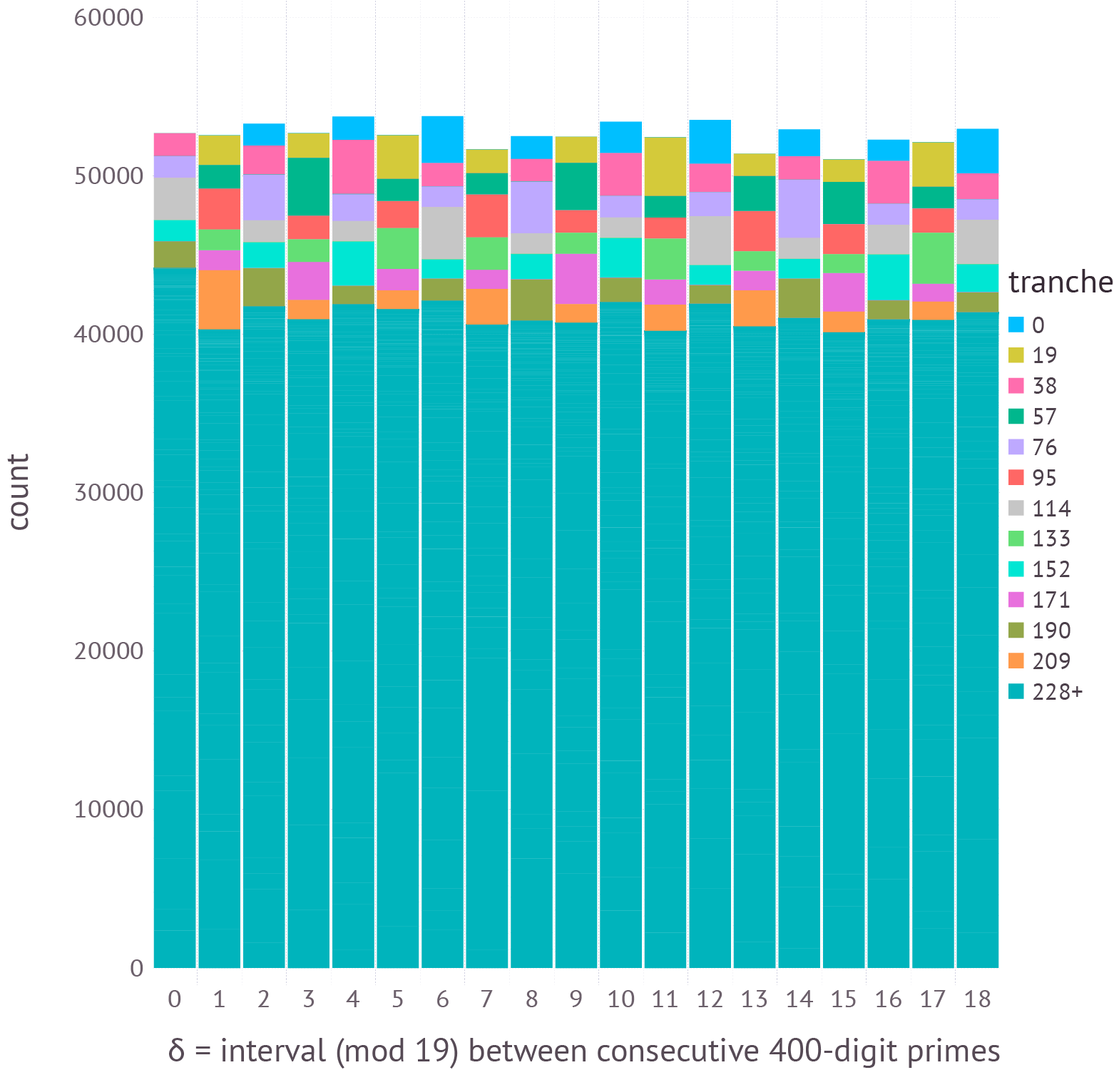
And the chronically unpopular class of intervals congruent to 0 mod 19 has finally caught up with its peers. Most of the height of the bars comes not from the dozen early tranches but from the hundreds of later ones representing intervals between 228 and 15,080 (all lumped together in the teal green area of the graph).
The experiments with large primes suggest a plausible surmise: As the size of the primes goes to infinity, all traces of correlations will fade to gray, and consecutive pairs of primes will be as random as rolls of an ideal die. But is it so? There are several reasons to be skeptical of this hypothesis. First, if we scale the modulus m along with the size of the primes—making it comparable in magnitude to the median gap between primes—the correlations may still show through. For my 40-digit sample, the median gap between primes is 66, so let’s look at the successive-pairs matrix mod 61. (To limit statistical noise, I did this computation with a sample of 10 million 40-digit primes rather than 1 million.)
Figure 25.

The stripes are back! Indeed, in addition to the familiar bright red stripes at intervals of 6, there’s a more diffuse pink-and-blue undulation with a period of 30. I would love to see a matrix for primes of 400 digits, which might well have even more complex features, with interacting waves at periods of 6, 30, and 210. Regrettably, I can’t show you that figure. The median gap between 400-digit primes is about 640, so we’d need to set m equal to a prime in this range, say 641. Filling that 641 × 641 matrix would require about a billion consecutive 400-digit primes, which is more than I’m prepared to calculate.
There are other reasons to doubt that the correlations disappear entirely as the primes grow larger. The comblike structure seen so clearly in Figures 21 and 23 suggests that rules of divisibility by small primes have a major influence on the distribution of large primes mod m—and this influence does not wane when the primes grow larger still. Furthermore, even when m is much smaller than the median inter-prime interval, the blue streak remains faintly visible. Here is the matrix for pairs of consecutive 400-digit primes mod 3:
                             1       2
                    1   248291  251128
                    2   251127  249453
Differences between on-diagonal and off-diagonal elements are much smaller than with eight-digit primes (compare Figure 3), but the discrepancies still don’t look like random variation.
To get a clearer picture of how the correlations vary as a function of the size of the primes, I set out to sample the sequence of primes over the entire range from 1-digit numbers to 400-digit numbers. In this project I decided to go Gauss one better: He tabulated primes by the chiliad (a group of 1,000), and I’ve been computing them by the myriad (a group of 10,000). To measure the correlations among primes mod m, I calculated the mean value of the diagonal elements of the matrix and the mean of the off-diagonal elements, then took the off/on ratio. If successive primes were totally uncorrelated, the ratio should converge to 1.
Figure 26 shows the result for 797 myriads of primes mod 3. The curve is concave upward, with a steep initial decline and then a much flatter segment. Starting at about 100 digits, there are samples with off/on ratios of less than 1, meaning that the diagonal is more densely populated than the off-diagonal regions. But even at 400 digits the majority of the ratios are still above 1. What are we looking at here? Does the curve slowly approach a ratio of 1, or is there a limiting value slightly greater than 1? Unfortunately, computational experiments will not give a definitive answer.
Figure 26.

The paper by Lemke Oliver and Soundararajan brings quite different tools to bear on this problem. Although they do some numerical exploration, their focus is on finding an analytic solution. The goal is a mathematical function or formula whose inputs are four positive integers: m is a modulus, a and b are congruence classes of primes mod m, and x is an upper limit on the size of the primes. The formula should tell us how often a is followed by b among all primes smaller than x. If we were in possession of such a formula, we could color in all the squares in the m × m successor matrix without ever having to compute the actual primes up to x.
Describing the behavior of all primes up to x is far more challenging than taking a sample of primes in the neighborhood of x. And the analytic approach is harder in other ways: It requires ideas rather than just cpu cycles. The reward is also potentially greater. The equation \(A = \pi r^2\) yields an exact truth about all circles, something no finite series of computations (with a finite approximation to \(\pi\)) can give us. There’s the promise not just of rigor but of insight.
Sadly, I’ve not yet been able to gain much insight from reading the analysis of Lemke Oliver and Soundararajan. The blame lies mainly with gaping holes in my knowledge of analytic number theory, but I think it’s also fair to say that the math gets pretty hairy at certain points in this discourse. The equation below constitutes the Main Conjecture of Lemke Oliver and Soundararajan. (I have made a minor change of notation and simplified one aspect of the equation: The original applies to sequences of r consecutive primes, but this version describes pairs only, i.e., \(r = 2\).)
\[\pi(x; m, a, b) = \frac{\mathrm{li}(x)}{\phi(m)^2}\left(1 + c_1(m; a, b)\frac{\log \log x}{\log x} + c_2(m; a, b) \frac{1}{\log x} + O\Big( \frac{1}{(\log x)^{7/4}} \Big) \right)\]
I think I understand enough of what’s going on here to at least offer a glossary. To the left of the equal sign, \(\pi(x; m, a, b)\) denotes a counting function; whereas \(\pi(x)\) counts the primes up to \(x\), \(\pi(x; m, a, b)\) is the number of pairs of consecutive primes mod \(m\) that fall into the congruence classes \(a\) and \(b\). To the right of the equal sign, the main coefficient \(\mathrm{li}(x) / \phi(m)^2\) is essentially the mean or expected number of pairs if the primes were distributed uniformly at random, with no correlations between successive primes; \(\mathrm{li}(x)\) is the logarithmic integral of \(x\), an approximation to \(\pi(x)\), and \(\phi(m)^2\) is the Euler totient function, which counts the square of the number of possible congruence classes for \(m\), or in other words the number of elements in the successor matrix.
The leading term inside the large parentheses is simply \(1\), and so it takes on the value of the main coefficient \(\mathrm{li}(x) / \phi(m)^2\); thus the mean number of pairs \((a, b)\) becomes the first approximation to the counting function. The three following terms act as corrections to this first approximation; for large \(x\) they should get progressively smaller, because \(\log \log x / \log x \gt 1 / \log x \gt 1 / (\log x)^{7/4}\) whenever \(x \gt e^e \approx 15\).
What about the coefficients of those three correction terms? The notation \(O(\cdot)\) for the smallest term indicates that we’re only going to worry about the term’s order of magnitude—which will be small for large \(x\). The coefficient \(c_1\) takes the following form in the case of \(r = 2\):
\[c_1(m; a, b) = \frac{1}{2} - \frac{\phi(m)}{2} (\#\{a \equiv b \bmod m\})\]
The expression \(\#\{a \equiv b \bmod m\}\) counts the number of cases where \(a\) and \(b\) lie in the same congruence class mod \(m\). Thus the effect of the term (if I understand correctly) is to reduce the overall count along the matrix diagonal, where \(a \equiv b \bmod m\).
As for coefficient \(c_2\), Lemke Oliver and Soundararajan remark that “in general, [it] seems complicated.” Indeed it does. And so this is the place where I should encourage those readers who want to know more to go read the original.
The complexity of the mathematical treatment leaves me feeling frustrated, but it’s hardly unusual for an easily stated problem to require a deep and difficult solution. I hang onto the hope that some of the technicalities will be brushed aside and the main ideas will emerge more clearly with further work. In the meantime, it’s still possible to explore a fascinating and long-hidden corner of number theory with the simplest of computational tools and a bit of graphics.
“God may not play dice with the universe, but something strange is going on with the prime numbers”—so said Paul Erdős and/or Mark Kac, though only with a little help from Carl Pomerance. The strangeness seems to be at its strangest when we play dice with the primes.
Addendum 2016-06-14. I noted above that the distribution of primes mod 7 seems flatter, or more nearly uniform, than the result of rolling a fair die. John D. Cook has taken a chi-squared test to the data and shows that the fit to uniform distribution is way too good to be the plausible outcome of a random process. His first post deals with the specific case of primes modulo 7; his second post considers other moduli.
Update 2020-09-07. The source code for this project was written in an version of Julia that is now long out of date, by a programmer who was just starting to learn the language. I have now written a more modern and streamlined version. It’s in a folder named primeafterprime2020 in the Github repository. There’s a new Jupyter notebook and also a version for Pluto.js, a new Julia-only notebook system that’s pretty cool.
References
Ash, Avner, Laura Beltis, Robert Gross, and Warren Sinnott. 2011. Frequencies of successive pairs of prime residues. Experimental Mathematics 20(4):400–411.
Chebyshev, Pafnuty Lvovich. 1853. Lettre de M. le Professeur Tchébychev à M. Fuss sur un nouveaux théorème relatif aux nombres premiers contenus dans les formes 4n + 1 et 4n + 3. Bulletin de la Class Physico-mathematique de l’Academie Imperiale des Sciences de Saint-Pétersbourg 11:208. Google Books
Cramér, Harald. 1936. On the order of magnitude of the difference between consecutive prime numbers. Acta Arithmetica 2:23–46. PDF
Derbyshire, John. 2002. Chebyshev’s bias.
Granville, Andrew. 1995. Harald Cramér and the distribution of prime numbers. Harald Cramér Symposium, Stockholm, 1993. Scandinavian Actuarial Journal 1:12–28. PDF
Granville, Andrew, and Greg Martin. 2004. Prime number races. arXiv
Hamza, Kais, and Fima Klebaner. 2012. On the statistical independence of primes. The Mathematical Scientist 37:97–105.
Klarreich, Erica. 2016. Mathematicians discover prime conspiracy. Quanta.
Knapowski, S., and P. Turán. 1977. On prime numbers ? 1 resp. 3 mod 4. In Number Theory and Algebra: Collected Papers Dedicated to Henry B. Mann, Arnold E. Ross, and Olga Taussky-Todd, pp. 157–165. Edited by Hans Zassenhaus. New York: Academic Press.
Ko, Chung-Ming. 2002. Distribution of the units digit of primes. Chaos Solitons Fractals 13(6):1295–1302.
Lamb, Evelyn. 2016. Peculiar pattern found in ‘random’ prime numbers. Nature doi:10.1038/nature.2016.19550.
Lemke Oliver, Robert J., and Kannan Soundararajan. 2016 preprint. Unexpected biases in the distribution of consecutive primes. arXiv
Odlyzko, Andrew, Michael Rubinstein, and Marek Wolf. 1999. Jumping champions. Experimental Mathematics 8(2):107–118.
Rubinstein, Michael, and Peter Sarnak. 1994. Chebyshev’s bias. Experimental Mathematics 3:173–197. Project Euclid
Tao, Terrence. Structure and randomness in the prime numbers. PDF
Very interesting discussion, thank you.
How practical is it to use distributed julia processing over the internet for this type of project? If you had volunteers who were willing to install julia and give you access on unused computers for a few days at a time, would that make bigger computational tasks significantly faster if the internet connections were fast enough? I’d be willing to discuss that.
Thanks for the suggestion. The only part of the process that requires significant computing resources is the generation of long sequences of consecutive large primes. That could certainly be done by the kind of volunteer organization you propose, and in fact I think it once was done: See bigprimes.net. But that project appears to be moribund, and perhaps with good reason. With current tradeoffs between cpu speed and network bandwidth, it’s usually better to compute primes than to download them.
Well, you could download the starting prime and then a list of successive distances.
While the math is very interesting, the quilt pattern idea made me think of the Bridges math art community. This might be a worthy topic for a Bridges paper, or at least pictures for the art exhibition — the math behind the art is a key consideration there.
I noticed you already have connections to the JMM, and their art galleries are hosted jointly with Bridges ones, so perhaps you’re already aware of Bridges?
(Disclaimer: I’m a first time participant in this year’s Bridges conference next month.)
I’m a big fan of Bridges, but I’ve never managed to get to the Conference. Saddened by the loss of Reza Sarhangi.
Just a note that your article was linked on a discussion of gapcoin, a cryptocurrency that finds prime gaps
https://bitcointalk.org/index.php?topic=822498