
Around 2006, my friend Dan Christensen created a fascinating picture of all the roots of all polynomials of degree ≤ 5 with integer coefficients ranging from -4 to 4:
Click on the picture for bigger view. Roots of quadratic polynomials are in grey; roots of cubics are in cyan; roots of quartics are in red and roots of quintics are in black. The horizontal axis of symmetry is the real axis; the vertical axis of symmetry is the imaginary axis. The big hole in the middle is centered at 0; the next biggest holes are at ±1, and there are also holes at ±i and all the sixth roots of 1.
You can see lots of fascinating patterns here, like how the roots of polynomials with integer coefficients tend to avoid integers and roots of unity - except when they land right on these points! You can see more patterns if you zoom in:

Now you see beautiful feathers surrounding the blank area around the point 1 on the real axis, a hexagonal star around \(\exp(i \pi/ 3)\), a strange red curve from this point to 1, smaller stars around other points, and more....
People should study this sort of thing! Let's define the Christensen set \(C_{d,n}\) to be the set of all roots of all polynomials of degree \(d\) with integer coefficients ranging from \(-n\) to \(n\). Clearly \(C_{d,n}\) gets bigger as we make either \(d\) or \(n\) bigger, and it becomes dense in the complex plane as \(n\) approaches \(\infty\), as long as \( d \ge 1\). We get all the rational complex numbers if we fix \(d \ge 1\) and let \( n \to \infty\), and we get all the algebraic complex numbers if let both \(d, n \to \infty \). Based on the above picture, there seem to be lots of interesting conjectures to make about what it does as \(d \to \infty\) for fixed \(n\).
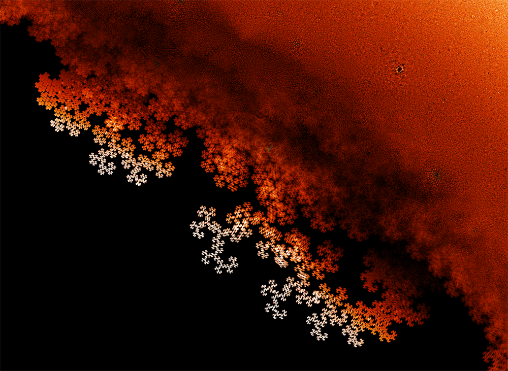
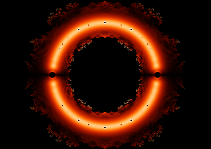
Inspired by the pictures above, Sam Derbyshire decided to to make a high resolution plot of some roots of polynomials. After some experimentation, he decided that his favorite were polynomials whose coefficients were all 1 or -1 (not 0). He made a high-resolution plot by computing all the roots of all polynomials of this sort having degree ≤ 24. That's \( 2^{24} \) polynomials, and about \( 24 \times 2^{24} \) roots — or about 400 million roots! It took Mathematica 4 days to generate the coordinates of the roots, producing about 5 gigabytes of data. He then used some Java programs to create this amazing image:

The coloring shows the density of roots, from black to dark red to yellow to white. The picture above is a low-resolution version of the original 90-megabyte file, which you can get here. We can zoom in to get more detail:

Note the holes at certain roots of unity and the feather-like patterns as we move inside the unit circle. To see these pattern, let's zoom in to certain regions, marked here:

Here's a closeup of the hole at 1:

Note the white line along the real axis. That's because lots more of these polynomials have real roots than nearly real roots.
Next, here's the hole at i:

And here's the hole at \( \exp(i \pi /4) = (1 + i)/\sqrt{2} \):

Note how the density of roots increases as we get closer to this point, but then suddenly drops off right next to it. Note also the subtle patterns in the density of roots.
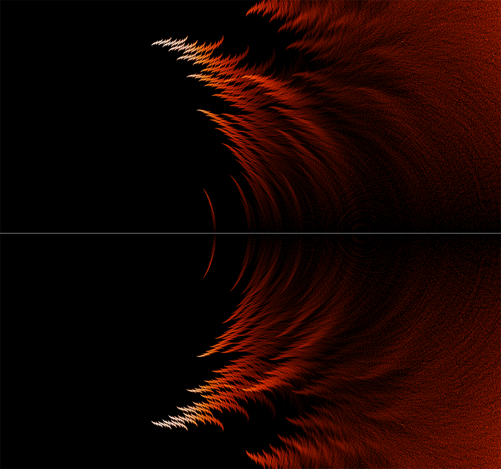
But the feathery structures as move inside the unit circle are even more beautiful! Here is what they look near the real axis — this plot is centered at the point 4/5:

They have a very different character near the point \( (4/5)i\):

But I think they're the most beautiful near the point \( (1/2)\exp(i/5)\). This image is almost a metaphor of how, in our study of mathematics, patterns emerge from confusion like sharply defined figures looming from the mist:

The patterns I've just showed you are tantalizing, and at first quite mysterious... but Jesse C. McKeown and Greg Egan figured out how to understand some of them during the discussion of "week285". The resulting story is quite beautiful! But this discussion was a bit hard to follow, since it involved smart people figuring out things as they went along. So, I doubt many people understood it---at least compared to the number of people who could understand it. Let me just explain one pattern here. Why does this region near \( \frac{1}{2}e^{i/5}\):
look so much like the fractal called a dragon?
Here's another, more relevant way to create a dragon. Take these two functions from the complex plane to itself:
$$ \displaystyle{ f_+ (x) = \frac{1+i}{2} x } $$
$$ \displaystyle{ f_- (x) = 1- \frac{1-i}{2} x } $$
Pick a point in the plane and keep hitting it with either of these functions: you can randomly make up your mind which to use each time. No matter what choices you make, you'll get a sequence of points that converges... and it converges to a point in the dragon! We can get all points in the dragon this way.
But where did these two functions come from? What's so special about them?
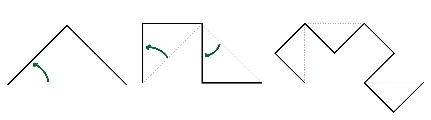
To get the specific dragon I just showed you, we need these specific functions. They have the effect of taking the horizontal line segment from the point 0 to the point 1, and mapping it to the two segments that form the simple picture shown at the far left here:
As we repeatedly apply them, we get more and more segments, which form the ever more fancy curves in this sequence.
But if all we want is some sort of interesting set of points in the plane, we don't need to use these specific functions. The most important thing is that our functions be contractions, meaning they reduce distances between points. Suppose we have two contractions \( f_+ \) and \( f_- \) from the plane to itself. Then there is a unique closed and bounded set \(D\) in the plane with
$$ D = f_+(D) \cup f_-(D) $$
Moreover, suppose we start with some point \(x\) in the plane and keep hitting it with \(f_+\) and/or \(f_-\), in any way we like. Then we'll get a sequence that converges to a point in \(S\). And even better, every point in \(S\) show up as a limit of a sequence like this. We can even get them all starting from the same \(x\). All this follows from a famous theorem due to John Hutchinson.
"Cute," you're thinking. "But what does this have to do with roots of polynomials whose coefficients are all 1 or -1?"
Well, we can get polynomials of this type by starting with the number 0 and repeatedly applying these two functions, which depend on a parameter \(z\):
$$ f_+(x) = 1 + z x $$
$$ f_-(x) = 1 - z x $$
For example:
$$ f_+(0) = 1 $$
$$ f_+(f_+(0)) = 1 + z $$
$$ f_-(f_+(f_+(0))) = 1 - z(1 + z) = 1 - z - z^2 $$
$$ f_+(f_-(f_+(f_+(0)))) = 1 + z(1 - z - z^2) = 1 - z - z^2 + z^3 $$
and so on. All these polynomials have constant term 1, never -1. But apart from that, we can get all polynomials with coefficients 1 or -1 using this trick. So, we get them all up to an overall sign — and that's good enough for studying their roots.
Now, depending on what \(z\) is, the functions \( f_+ \) and \( f_- \) will give us different generalized dragon sets. We need \( |z| \lt 1 \) for these functions to be contraction mappings. Given that, we get a generalized dragon set in the way I explained. Let's call it \(D_z\) to indicate that it depends on \(z\).
Greg Egan drew some of these sets \(D_z\). Here's one that looks like a dragon:
Here's one that looks more like a feather:
The words 'looks like' are weasel words, because I don't know the precise theorem. If you look at Sam's picture again:
you'll see a lot of 'haze' near the unit circle, which is where \( f_+ \) and \( f_- \) cease to be contraction mappings. Outside the unit circle — well, I don't want to talk about that now! But inside the unit circle, you should be able to see that I'm at least roughly right. For example, if we zoom in near \( z = 0.372 - .542 i\), we get dragons:
which look at least roughly like this:
In fact they should look very much like this, but I'm too lazy to find the point \(z = 0.372 - .542 i\) and zoom in very closely to that point in Sam's picture, to check!
Similarly, near the point \(0.8 + 0.2 i\), we get feathers:
that look a lot like this:
Again, it would be more convincing if I could exactly locate the point \(0.8 + 0.2 i\) and zoom in there.
There are lots of questions left to answer, like "What about all the black regions in the middle of Sam's picture?" and "what about those funny-looking holes near the unit circle?" But the most urgent question is this:
If you take the set Sam Derbyshire drew and zoom in near the point z, why should it look like the generalized dragon set Dz?
And the answer was discovered by 'some guy on the street' — our pseudonymous, nearly anonymous friend. It's related to something called the Julia–Mandelbrot correspondence. I wish I could explain it clearly, but I don't understand it well enough to do a really convincing job. So, I'll just muddle through by copying Greg Egan's explanation.
First, let's define a Littlewood polynomial to be one whose coefficients are all 1 or -1.
We have already seen that if we take any number \( z\), then we get the image of \(z\) under all the Littlewood polynomials of degree \(n\) by starting with the point \( x = 0\) and applying these functions over and over: $$ f_+(x) = 1 + z x $$ $$ f_-(x) = 1 - z x $$ a total of \( n+1 \) times.
Moreover, we have seen that as we keep applying these functions over and over to \( x = 0\), we get sequences that converge to points in the generalized dragon set \(D_z\).
So, \(D_z\) is the set of limits of sequences that we get by taking the number \(z\) and applying Littlewood polynomials of larger and larger degree.
Now, suppose 0 is in \(D_z\). Then there are Littlewood polynomials of large degree applied to \( z \) that come very close to 0. We get a picture like this:
where the arrows represent different Littlewood polynomials being applied to \( z\). If we zoom in close enough that a linear approximation is good, we can see what the inverse image of 0 will look like under these polynomials:
It will look the same! But these inverse images are just the roots of the Littlewood polynomials. So the roots of the Littlewood polynomials near \( z \) will look like the generalized dragon set \( D_z\).
As Egan put it:
But if we grab all these arrows:
and squeeze their tips together so that they all map precisely to 0 — and if we're working in a small enough neighbourhood of 0 that the arrows don't really change much as we move them — the pattern that imposes on the tails of the arrows will look a lot like the original pattern:
There's a lot more to say, but I think I'll stop soon. I just want to emphasize that all this is modeled after the incredibly cool relationship between the Mandelbrot set and Julia sets. It goes like this;
Consider this function, which depends on a complex parameter \( z\): $$ f(x) = x^2 + z $$
If we fix \( z\), this function defines a map from the complex plane to itself. We can start with any number \(x\) and keep applying this map over and over. We get a sequence of numbers. Sometimes this sequence shoots off to infinity and sometimes it doesn't. The boundary of the set where it doesn't is called the Julia set for this number \( z\).
On the other hand, we can start with \( x = 0\), and draw the set of numbers \(z\) for which the resulting sequence doesn't shoot off to infinity. That's called the Mandelbrot set.
Here's the cool relationship: in the vicinity of the number \(z\), the Mandelbrot set tends to look like the Julia set for that number \(z\). This is especially true right at the boundary of the Mandelbrot set.
For example, the Julia set for $$ z = -0.743643887037151 + 0.131825904205330 i$$ looks like this:
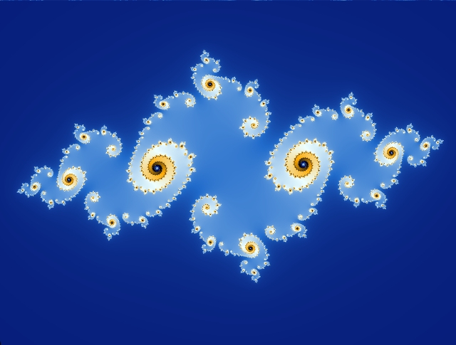
while this:

is a tiny patch of the Mandelbrot set centered at the same value of \(z\). They're shockingly similar!
This is why the Mandelbrot set is so complicated. Julia sets are already very complicated. But the Mandelbrot set looks like a lot of Julia sets! It's like a big picture of someone's face made of little pictures of different people's faces.
Here's a great picture illustrating this fact. As with all the pictures here, you can click on it for a bigger view:
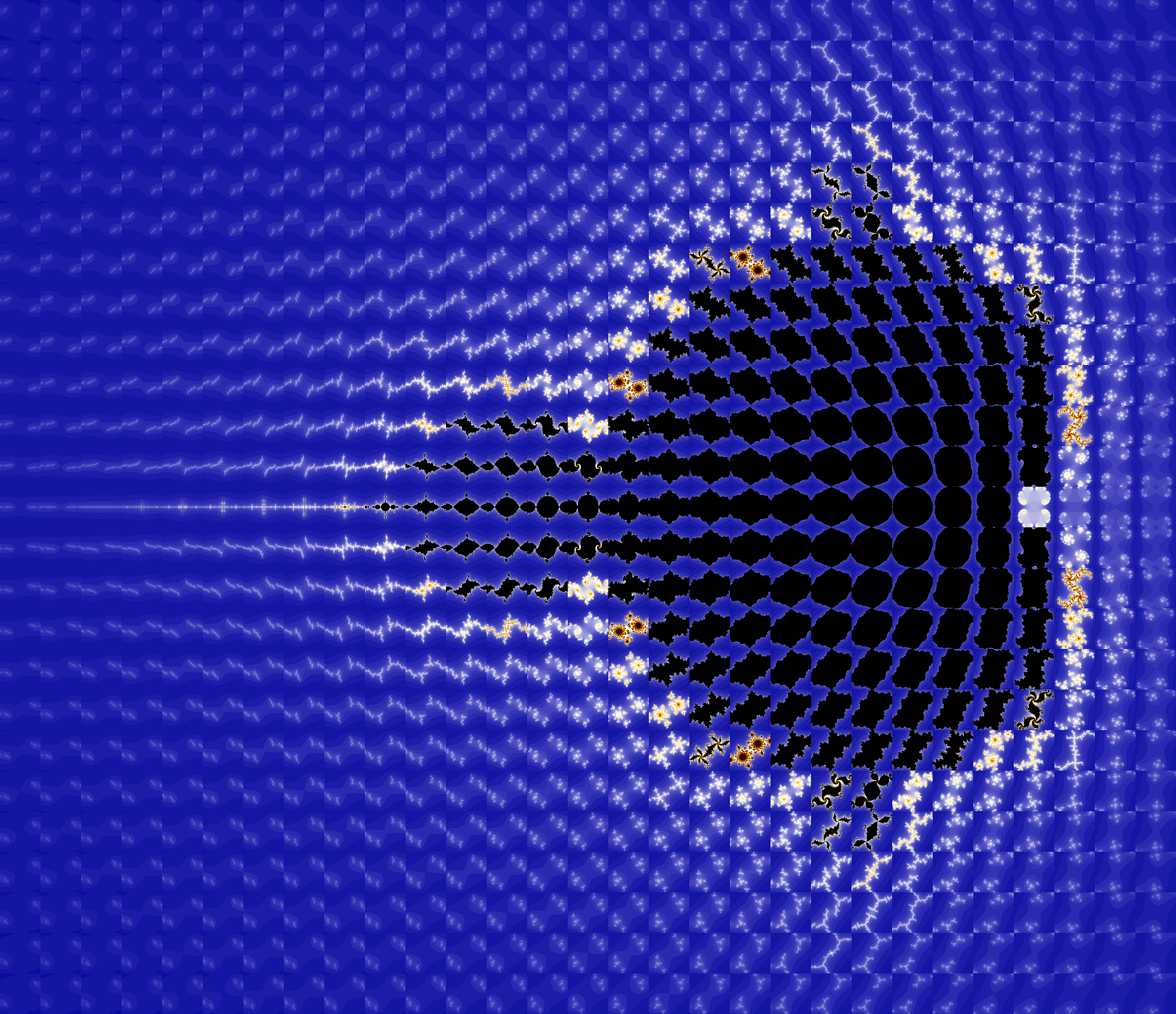
But this one you really must click on! It's a big picture made of lots of little pictures of Julia sets for various values of \(z\)... but it mimics the Mandelbrot set. You'll notice that the Mandelbrot set is the set of numbers \(z\) whose Julia sets are connected. Those Julia sets are the black blobs. When \(z\) leaves the Mandelbrot set, its Julia set falls apart into dust: that's the white stuff.
For an even better view of this phenomenon, try this:
You can zoom into the Mandelbrot set and see the corresponding Julia set at various values of \(z\). For example, here's the Julia set at \(z = -0.689494949 - 0.462323232 i\):
and here's a tiny piece of Mandelbrot set near that point:
So, the Mandelbrot set is like an illustrated catalog of Julia sets. Similarly, it seems the set of roots of Littlewood polynomials (up to a given degree) resembles a catalog of generalized dragon sets. However, making this into a theorem would require me to make precise many things I've glossed over, and I don't know how yet.
For more on this subject, see:
Greg Egan, Littlewood applet. An interactive webpage that lets you explore regions of the Derbyshire set and compare them to the corresponding dragons.
Odlyzko and Poonen proved some interesting things about the set of all roots of all polynomials with coefficients 0 or 1. If we define a fancier Christensen set Cd,p,q to be the set of roots of all polynomials of degree d with coefficients ranging from \(p\) to \(q\), Odlyzko and Poonen are studying \(C_{d,0,1}\) in the limit \(d \to \infty\). They mention some known results and prove some new ones: this set is contained in the half-plane \(\mathrm{Re}(z) \lt 3/2\) and contained in the annulus \(1/\Phi \lt |z| \lt \Phi\) where \(\Phi \) is the golden ratio \( (\sqrt{5} + 1)/2\). In fact they trap it, not just between these circles, but between two subtler curves. They also show that the closure of this set is path connected but not simply connected.