Following a Select Statement Through Postgres Internals

Captain Nemo takes Professor Aronnax on a tour
of the engine room, a fascinating description
of future technology from an 1870 perspective.
This is the third of a series of four posts based on a presentation I did at the Barcelona Ruby Conference called “20,000 Leagues Under ActiveRecord.” (posts: one two four and video).
Preparing for this presentation over the Summer, I decided to read through parts of the PostgreSQL C source code. I executed a very simple select statement and watched what Postgres did with it using LLDB, a C debugger. How did Postgres understand my query? How did it actually find the data I was looking for?
This post is an informal journal of my trip through the guts of Postgres. I’ll describe the path I took and what I saw along the way. I’ll use a series of simple, conceptual diagrams to explain how Postgres executed my query. In case you understand C, I’ll also leave you a few landmarks and signposts you can look for if you ever decide to hack on Postgres internals.
In the end, the Postgres source code delighted me. It was clean, well documented and easy to follow. Find out for yourself how Postgres works internally by following me on a journey deep inside a tool you use everyday.
Finding Captain Nemo
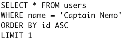
Here’s the example query from the first half of my presentation; we’ll follow Postgres as it searches for Captain Nemo:

Professor Aronnax and Captain Nemo
plot the course of the Nautilus.
Finding a single name in string column like this should be straightforward, shouldn’t it? We’ll hold tightly onto this select statement while we explore Postgres internals, like a rope deep sea divers use to find their way back to the surface.
The Big Picture
What does Postgres do with this SQL string? How does it understand what we meant? How does it know what data we are looking for?
Postgres processes each SQL command we send it using a four step process.
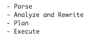
In the first step, Postgres parses our SQL statement and converts it into a series of C memory structures, a parse tree. Next Postgres analyzes and rewrites our query, optimizing and simplifying it using a series of complex algorithms. After that, Postgres generates a plan for finding our data. Like an obsessive compulsive person who won’t leave home without every suitcase packed perfectly, Postgres doesn’t run our query until it has a plan. Finally, Postgres actually executes our query. In this presentation I’ll briefly touch on the first three topics, and then focus more on the last step: Execute.
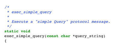
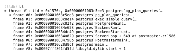
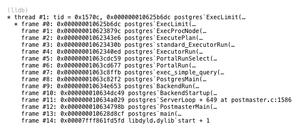
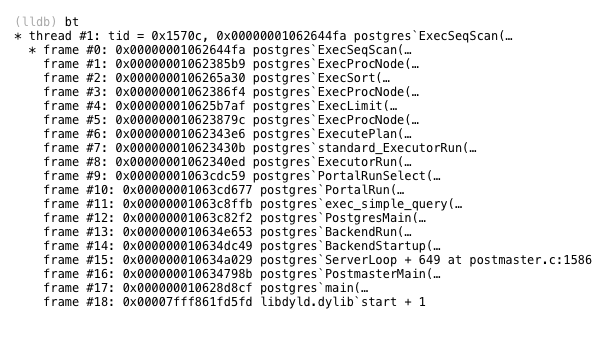
The C function inside of Postgres that implements this 4 step process is called exec_simple_query. You can find a link to it below, along with an LLDB backtrace which gives some context about exactly when and how Postgres calls exec_simple_query.

Parse
How does Postgres understand the SQL string we sent it? How does it make sense of the SQL keywords and expressions in our select statement? Through a process called parsing, Postgres converts our SQL string into an internal data structure it understands, the parse tree.
It turns out that Postgres uses the same parsing technology that Ruby does, a parser generator called Bison. Bison runs during the Postgres C build process and generates parser code based on a series of grammar rules. The generated parser code is what runs inside of Postgres when we send it SQL commands. Each grammar rule is triggered when the generated parser finds a corresponding pattern or syntax in the SQL string, and inserts a new C memory structure into the parse tree data structure.
I won’t take the time today to explain how parsing algorithms work in detail. If you’re interested in that sort of thing, I’d suggest taking a look at my book Ruby Under a Microscope. In Chapter One I go through a detailed example of the LALR parse algorithm used by Bison and Ruby. Postgres parses SQL statements in exactly the same way.
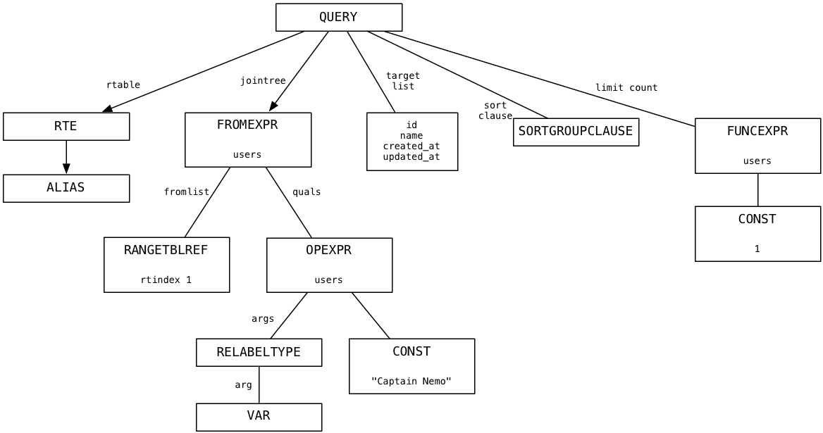
Using LLDB and enabling some C logging code, I observed the Postgres parser produce this parse tree for our Captain Nemo query:
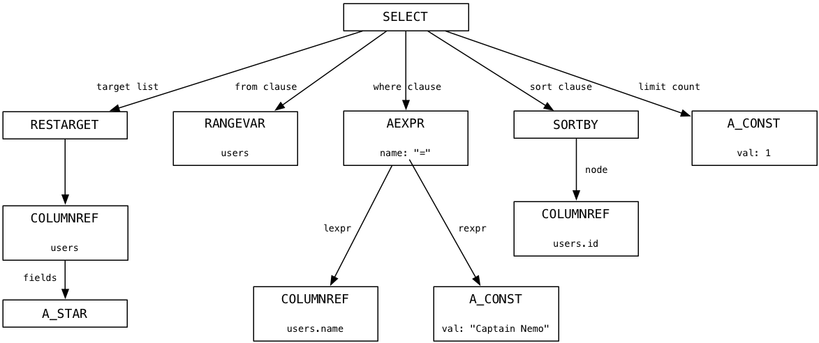
At the top is a node representing the entire SQL statement, and below that are child nodes or branches that represent the different portions of the SQL statement syntax: the target list (a list of columns), the from clause (a list of tables), the where clause, the sort order and a limit count.
If you want to learn more about how Postgres parses SQL statements, follow the flow of control down from exec_simple_query through another C function called pg_parse_query.
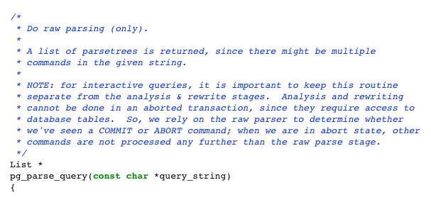

As you can see there are many helpful and detailed comments in the Postgres source code that not only explain what is happening but also point out important design decisions.
All That Hard Work For Nothing
The parse tree above should look familiar - it’s almost precisely the same as the abstract syntax tree (AST) we saw ActiveRecord create earlier. Recall from the first half of the presentation ActiveRecord generated our Captain Nemo select statement when we executed this Ruby query:
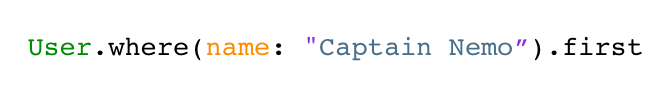
We saw that ActiveRecord internally created an AST when we called methods such as where and first. Later (see the second post), we watched as the Arel gem converted the AST into our example select statement using an algorithm based on the visitor pattern.
Thinking about this, it’s ironic that the first thing Postgres does with your SQL statement is convert it from a string back into an AST. Postgres’s parse process reverses everything ActiveRecord did earlier; all of that hard work the Arel gem did was for nothing! The only reason for creating the SQL string at all was to communicate with Postgres over a network connection. Once Postgres has the string, it converts it back into an AST, which is a much more convenient and useful way of representing queries.
Learning this you might ask: Is there a better way? Is there some way of conceptually specifying the data we want to Postgres without writing a SQL statement? Without learning the complex SQL language or paying the performance overhead of using ActiveRecord and Arel? It seems like a waste of time to go to such lengths to generate a SQL string from an AST, just to convert it back to an AST again. Maybe we should be using a NoSQL database solution instead?
Of course, the AST Postgres uses is much different from the AST used by ActiveRecord. ActiveRecord’s AST was comprised of Ruby objects, while Postgres’s AST is formed of a series of C memory structures. Same idea but very different implementations.
Analyze and Rewrite
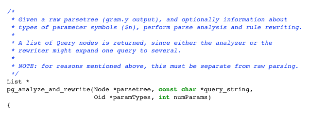
Once Postgres has generated a parse tree, it then converts it into a another tree structure using a different set of nodes. This is known as the query tree. Returning to the exec_simple_query C function, you can see it next calls another C function pg_analyze_and_rewrite.

Waving my hands a bit and glossing over many important details, the analyze and rewrite process applies a series of sophisticated algorithms and heuristics to try to optimize and simplify your SQL statement. If you had executed a complex select statement with sub-selects and multiple inner and outer joins, then there is a lot of room for optimization. It’s quite possible that Postgres could reduce the number of sub-select clauses or joins to produce a simpler query that runs faster.
For our simple select statement, here’s the query tree that pg_analyze_and_rewrite produces:
I don’t pretend to understand the detailed algorithms behind pg_analyze_and_rewrite. I simply observed that for our example the query tree largely resembled the parse tree. This means the select statement was so straightforward Postgres wasn’t able to simplify it further.
Plan
The last step Postgres takes before starting to execute our query is to create a plan. This involves generating a third tree of nodes that form a list of instructions for Postgres to follow. Here’s the plan tree for our select statement.
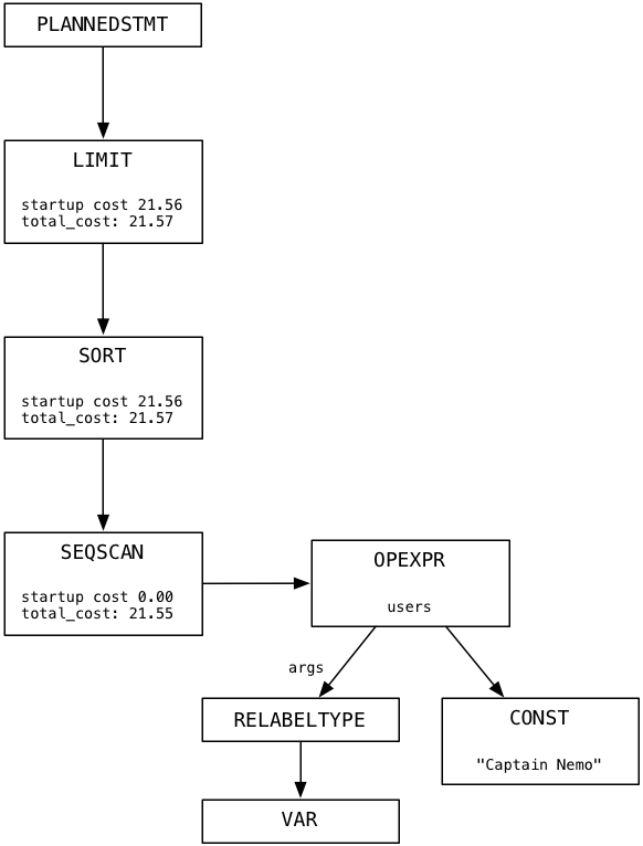
Imagine that each node in the plan tree is a machine or worker of some kind. The plan tree resembles a pipeline of data or a conveyor belt in a factory. In my simple example there is only one branch in the tree. Each node in the plan tree takes some the output data from the node below, processes it, and returns results as input to the node above. We’ll follow Postgres as it executes the plan in the next section.
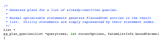
The C function that starts the query planning process is called pg_plan_queries.
Note the startup_cost and total_cost values in each plan node. Postgres uses these values to estimate how long the plan will take to complete. You don’t have to use a C debugger to see the execution plan for your query. Just prepend the SQL EXPLAIN command to your query, like this:

This is a powerful way to understand what Postgres is doing internally with one of your queries, and why it might be slow or inefficient - despite the sophisticated planning algorithms in pg_plan_queries.
Executing a Limit Plan Node
By now, Postgres has parsed your SQL statement and converted it back into an AST. Then it optimized and rewrote your query, possibly in a simpler way. Third, Postgres wrote a plan which it will follow to find and return the data you are looking for. Finally it’s time for Postgres to actually execute your query. How does it do this? It follows the plan, of course!
Let’s start at the top of the plan tree and move down. Skipping the root node, the first worker that Postgres uses for our Captain Nemo query is called Limit. The Limit node, as you might guess, implements the LIMIT SQL command, which limits the result set to the specified number of records. The same plan node also implements the OFFSET command, which starts the result set window at the specified row.

The first time Postgres calls the Limit node, it calculates what the limit and offset values should be, because they might be set to the result of some dynamic calculation. In our example, offset is 0 and limit is 1.
Next, the Limit plan node repeatedly calls the subplan, in our case Sort, counting until it reaches the offset value:
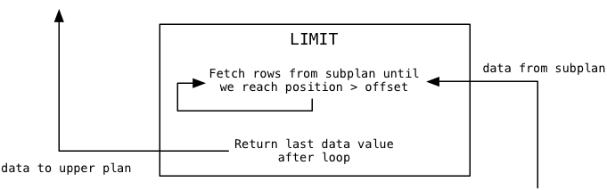
In our example the offset value is zero, so this loop will load the first data value and stop iterating. Then Postgres returns the last data value loaded from the subplan to the calling or upper plan. For us, this will be that first value from the subplan.
Finally when Postgres continues to call the Limit node, it will pass the data values through from the subplan one at a time:
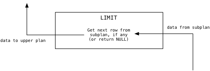
In our example, because the limit value is 1 Limit will immediately return NULL indicating to the upper plan there is no more data available.
Postgres implements the Limit node using code in a file called nodeLimit.c
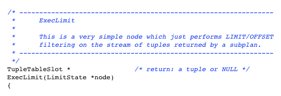
You can see the Postgres source code uses words such as tuple (a set a values, one from each column) and subplan. The subplan in this example is the Sort node, which appears below Limit in the plan.
Executing a Sort Plan Node
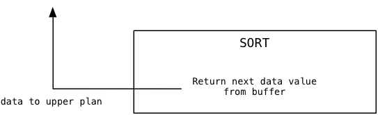
Where do the data values Limit filters come from? From the Sort plan node that appears under Limit in the plan tree. Sort loads data values from its subplan and returns them to its calling plan, Limit. Here’s what Sort does when the Limit node calls it for the first time, to get the first data value:
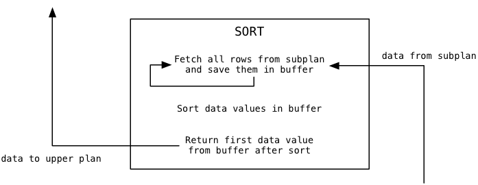
You can see that Sort functions very differently from Limit. It immediately loads all of the available data from the subplan into a buffer, before returning anything. Then it sorts the buffer using the Quicksort algorithm, and finally returns the first sorted value.
For the second and subsequent calls, Sort simply returns additional values from the sorted buffer, and never needs to call the subplan again:
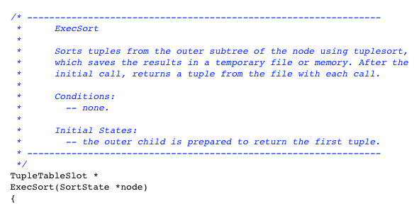
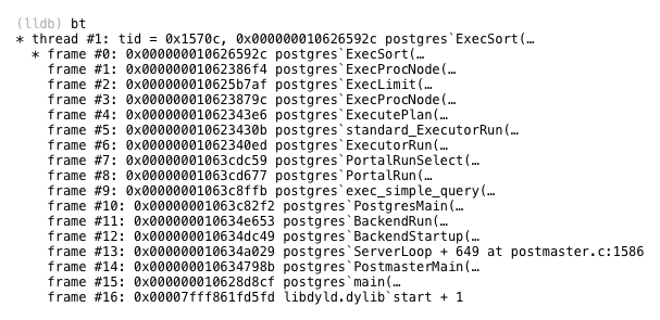
The Sort plan node is implemented by a C function called ExecSort:
Executing a SeqScan Plan Node
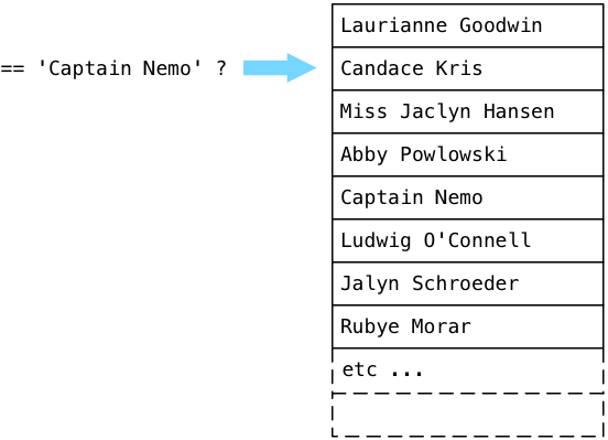
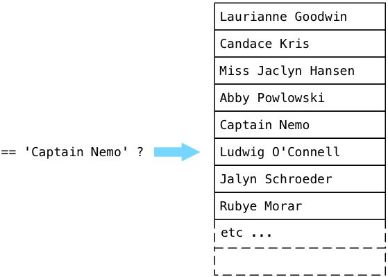
Where does ExecSort get its values? From its subplan, or the SeqScan node that appears at the bottom of the plan tree. SeqScan stands for sequence scan, which means to look through the values in a table, returning values that match a given filter. To understand how the scan works with our filter, let’s step through an imaginary users table filled with fake names, looking for Captain Nemo.
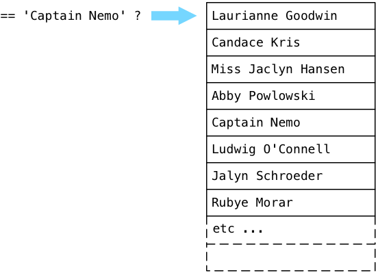
Postgres starts at the first record in a table (known as a relation in the Postgres source code) and executes the boolean expression from the plan tree. In simple terms, Postgres asks the question: “Is this Captain Nemo?” Because Laurianne Goodwin is not Captain Nemo, Postgres steps down to the next record.
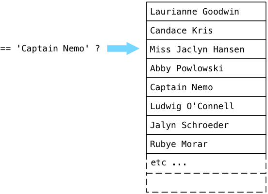
No, Candace is also not Captain Nemo. Postgres continues:
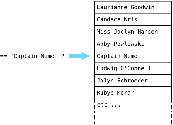
… and eventually finds Captain Nemo!
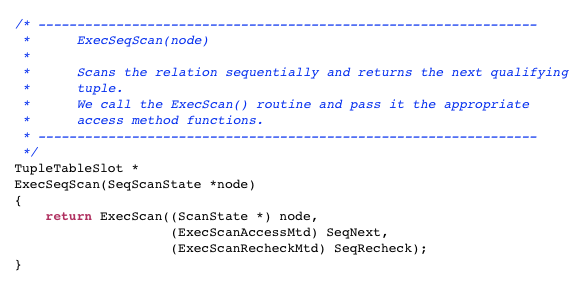
Postgres implements the SeqScan node using a C function called ExecSeqScan.
What Are We Doing Wrong?
Now we’re done! We’ve followed a simple select statement all the way through the guts of Postgres, and have seen how it was parsed, rewritten, planned and finally executed. After executing many thousands of lines of C code, Postgres has found the data we are looking for! Now all Postgres has to do is return the Captain Nemo string back to our Rails application and ActiveRecord can create a Ruby object. We can finally return to the surface of our application.
But Postgres doesn’t stop! Instead of simply returning, Postgres continues to scan through the users table, even though we’ve already found Captain Nemo:

While returning from the South Pole, the air
supply inside the Nautilus began to run out.
What’s going on here? Why is Postgres wasting its time, continuing to search even though it’s already found the data we’re looking for?
The answer lies farther up the plan tree in the Sort node. Recall that in order to sort all of the users, ExecSort first loads all of the values into a buffer, by calling the subplan repeatedly until there are no values left. That means that ExecSeqScan will continue to scan to the end of the table, until it has all of the matching users. If our users table contained thousands or even millions of records (imagine we work at Facebook or Twitter), ExecSeqScan will have to loop over every single user record and execute the string comparison for each one. This is obviously inefficient and slow, and will get slower as more and more user records are added.
If we have only one Captain Nemo record, then ExecSort will “sort” just that single matching record, and ExecLimit will pass that single record through its offset/limit filter… but only after ExecSeqScan has iterated over all of the names.
Next Time
How do we fix this problem? What should we do if our SQL queries on the users table take more and more time to execute? The answer is simple: we create an index.
In the next and final post in this series we’ll learn how to create a Postgres index and to avoid the use of ExecSeqScan. More importantly, I’ll show you what a Postgres index looks like: how it works and why it speeds up queries like this one.


