Edit: Part 2 of this post can be found here, and part 3 here. Most of the code used in these posts is available here.
Disclaimer
In this post I refer to lyrics of certain bands as being "Metal". I know some people have strong feelings about how genres are defined, and would probably disagree with me about some of the bands I call metal in this post. I call these band "Metal" here for the sake of brevity only, and I apologise in advance.
Introduction
Natural language is ubiquitous. It is all around us, and the rate at which it is produced in written, stored form is only increasing. It is also quite unlike any sort of data I have worked with before.
Natural language is made up of sequences of discrete characters arranged into hierarchical groupings: words, sentences and documents, each with both syntactic structure and semantic meaning.
Not only is the space of possible strings huge, but the interpretation of a small sections of a document can take on vastly different meanings depending on what context surround it.
These variations and versatility of natural language are the reason that it is so powerful as a way to communicate and share ideas.
In the face of this complexity it is not surprising that understanding natural language, in the same way humans do, with computers is still a unsolved problem. That said, there are an increasing number of techniques that have been developed to provide some insight into natural language. They tend to start by making simplifying assumptions about the data, and then using these assumptions convert the raw text into a more quantitative structure, like vectors or graphs. Once in this form, statistical or machine learning approaches can be leveraged to solve a whole range of problems.
I haven't had much experience playing with natural language, so I decided to try out a few techniques on a dataset I scraped from the internet: a set of heavy metal lyrics (and associated genres).
The Data
To get the lyrics, I scraped www.darklyrics.com. While darklyrics doesn't have a robots.txt file, I tried to be gentle with my requests. After cleaning the data up, identifying the languages and splitting albums into songs, we are left with a dataset containing lyrics to 222,623 songs from 7,364 bands spread over 22,314 albums.
Before anyone asks, I have no intention of releasing either the raw lyric files or the code used to scrape the website. I collected the lyrics for my own entertainment, and it would be too easy for someone to use this data to copy darklyrics. If people are interested I may release some n-gram data of the corpus.
Once we have the data, there are a huge number of ways to represent it in numerical form. For example, taking 100 of the more popular band from the dataset, we look at all the lyrics for the band and ask what fraction of the words are swear words? We can also look what the readability of their lyrics, giving us a measure of how complex the language used is (where complexity is defined in terms of the number of syllables each word has). Ploting one against the other we get the following:
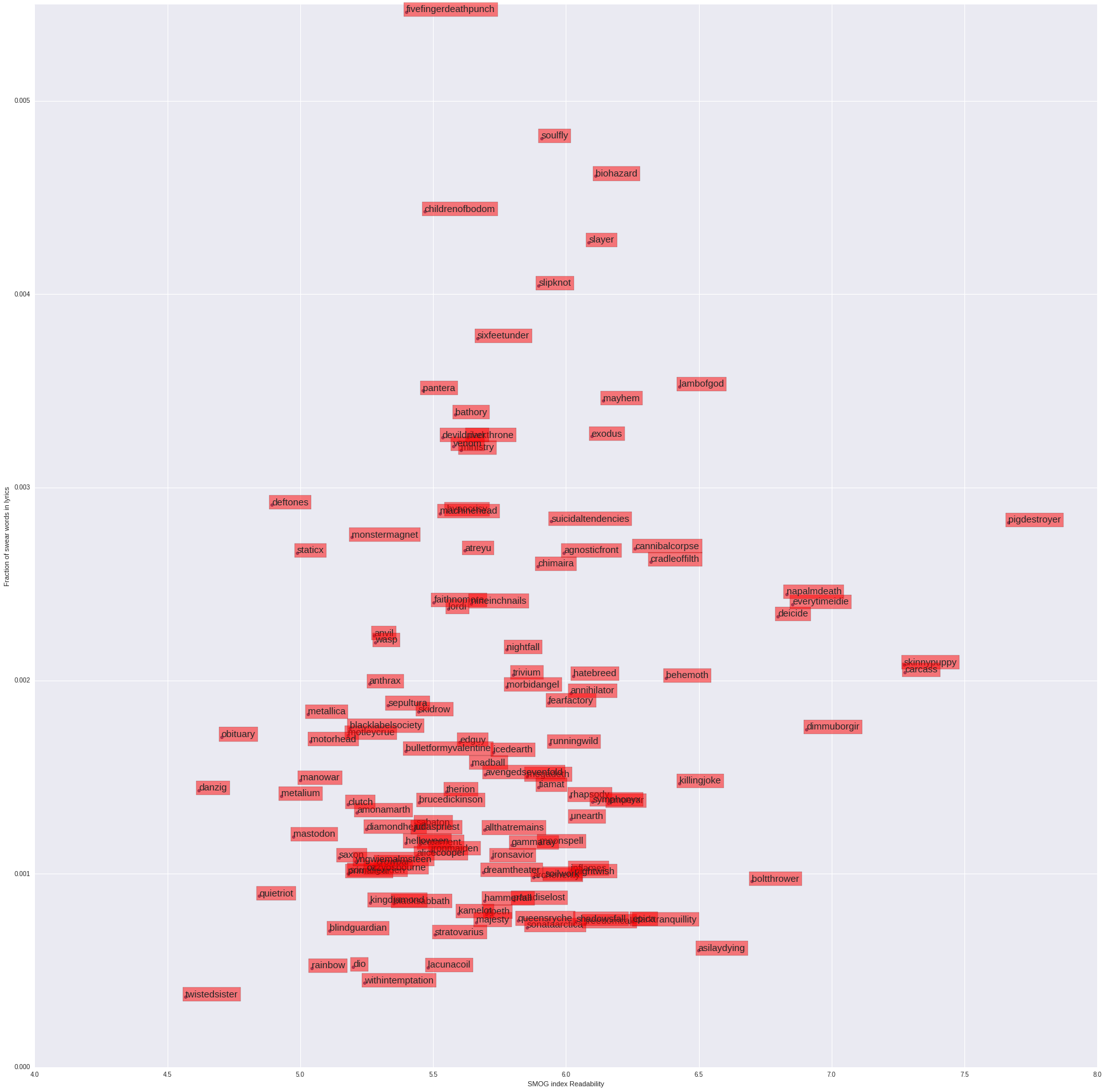
As you can see, Five Finger Death Punch have the highest number of swear words in their lyrics, and Pig Destroyer have the most complex wordplay. It also suggests that bands that swear more seem to use more complex words.
While this is an interesting way to represent the bands, it is limited in what it captures. In what follows, I'm going to explore more general ways we can looking at natural language, focusing on the "bag-of-words" model.
A "bag-of-words" model is one where we only care about the frequencies with which each word appears in the text of a document. In other words we throw away all information about the relative ordering of words. This approach obviously loses some information about the document being analyses. For example, the phrases "dog bites man" and "man bites dog" would end up with the same representation, despite referring to very different events. However, we do capture some information about the phrases, namely that both of them refer to a "dog" and to a "man". This suggests that in looking at word frequencies we are capturing some information about the "topic" of the models.
First Look
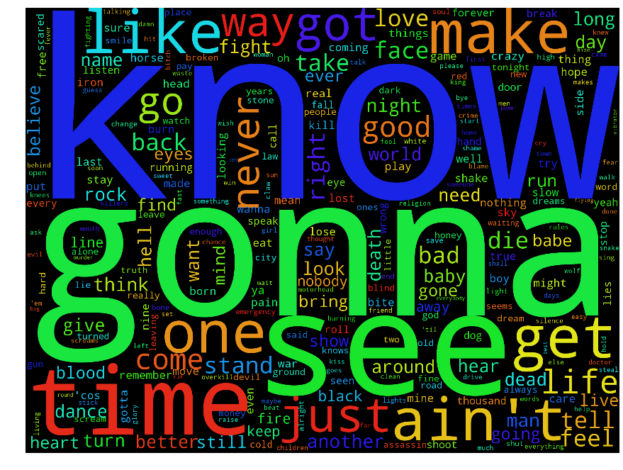
A good starting point when exploring text data is looking at the word frequencies of the whole text, and a nice way to visualise this is with a word cloud/tag clound, an image of the most frequently used words, with the size of each word adjusted to be proportional to the frequency of that words occurrence. As it happens, there is a nice package in python called word_cloud that allows me to produce one for the entire metal lyrics corpus:
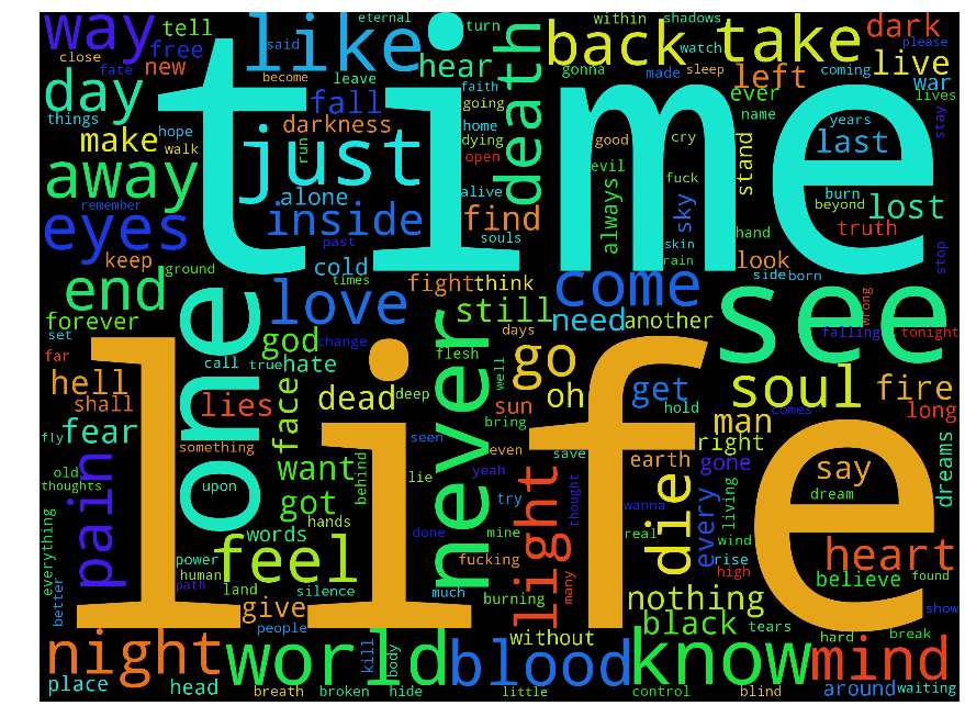
where I have removed the most common words the English language (known as "stop words").
We are starting to see some patterns emerge when we look at the cloud, and I feel like I could tell a story about what's happening. Metal lyrics seem focused on "time" and "life", with a healthy dose of "blood", "pain" and "eyes" thrown in. Even without knowing much about the genre, this is what you might expect.
It is worth stepping back and thinking about what we are trying to achieve by plotting this. We are making the assumption that the words that occur most frequently are important to the type of document being analysed. Now, the word "important" here is deliberately vague. It might refer to the topic being described by the lyrics, the style the lyrics are written in or something else.
As users of the English language, we can pick out "interesting" words just by eyeballing the word cloud. We get a feeling for the content of the documents just by prominence of the words "night", "pain" and "death". The word "see" also appears prominently in the word cloud, but isn't as interesting as the word "hell" or "blood", which appear less frequently in the lyrics. My feeling is that our prior experience of the English language guides our search. We know that the word "see" is usually common, but the words "death" are not, so we interpret it as important. Can we quantify this feeling?
One approach might be to look at how the relative frequency of words change between the metal lyrics and the English language in general. To do this we need some sort of measure of what "standard" English looks like, and given I'm using NLTK for text processing, an easy comparison is to the brown corpus, a collection of documents published in 1961 covering a range of different genres (although it should be pointed out, no lyrics).
To make a comparison between the two corpora, I define an arbitrary measure of "Metalness", \(M_{w}\) for each word \({w}\),
where \(N^{metal}_{w}\) is the frequency of occurrences of word \(w\) in my corpus of metal lyrics and \(N^{brown}_{w}\) is the frequency of occurrences of word \(w\) in the Brown corpus. To prevent us being skewed by rare words, we take only words which occur at least five times in each corpus.
The top and bottom 20 metal words are shown in the table below, along with their "Metalness".
Most Metal Words
| Rank | Word | Metalness |
|---|---|---|
| 1 | burn | 3.81 |
| 2 | cries | 3.63 |
| 3 | veins | 3.59 |
| 4 | eternity | 3.56 |
| 5 | breathe | 3.54 |
| 6 | beast | 3.54 |
| 7 | gonna | 3.53 |
| 8 | demons | 3.53 |
| 9 | ashes | 3.51 |
| 10 | soul | 3.40 |
| 11 | sorrow | 3.40 |
| 12 | sword | 3.38 |
| 13 | goodbye | 3.28 |
| 14 | dreams | 3.28 |
| 15 | gods | 3.24 |
| 16 | pray | 3.22 |
| 17 | reign | 3.15 |
| 18 | tear | 3.12 |
| 19 | flames | 3.12 |
| 20 | scream | 3.11 |
Least Metal Words
| Rank | Word | Metalness |
|---|---|---|
| 1 | particularly | -6.47 |
| 2 | indicated | -6.32 |
| 3 | secretary | -6.29 |
| 4 | committee | -6.16 |
| 5 | university | -6.09 |
| 6 | relatively | -6.08 |
| 7 | noted | -5.85 |
| 8 | approximately | -5.75 |
| 9 | chairman | -5.69 |
| 10 | employees | -5.67 |
| 11 | attorney | -5.66 |
| 12 | membership | -5.64 |
| 13 | administrative | -5.61 |
| 14 | considerable | -5.60 |
| 15 | academic | -5.51 |
| 16 | literary | -5.49 |
| 17 | agencies | -5.48 |
| 18 | measurements | -5.47 |
| 19 | fiscal | -5.45 |
| 20 | residential | -5.45 |
You can explore the full the Metalness of words here, where I've plotted the Metalness of all 10,000 words against word length in a d3 plot. Hover over each point to get the measured of the words. It appears that the longer a word is, on average the less metal it is.
Of course, this is a slightly unfair comparison. It is not too much to believe that not just the content of the documents we compare affects the word frequency, but also the type of the document being compared. A relevant example would be that a song about a brutal murder would have a different word count to a news article on the same murder. A better measure of what constitutes "Metalness" would have been a comparison with lyrics of other genres, unfortunately I don't have any of these to hand.
As a quick measure of the difference in style between the two corpora, we can look at how the distribution of parts of speech vary between them.
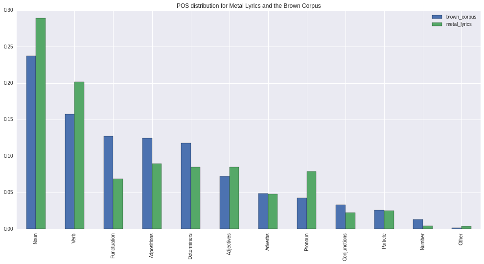
Here we can see that Metal lyrics focus much more on nouns, verbs and pronouns, whereas the brown corpus has far more adpositions and determiners. One explanation might be that lyrics are focused more fragmented descriptions which have been shortened to fit within the structure of a song, whereas the brown corpus contained news reports and similar, where any nouns and verbs descriptions needed to be placed in a wider context and related to other nouns and verbs, and to do so requires adpositions and determiners. Although, this is pure speculation and I may well be missing a simpler explanation.
Examplehead
Let us focus on three example bands: Motorhead, Machinehead and Diamondhead. Below I plot the absolute word clouds of each of the bands. I leave it as an exercise to the reader to work out which wordcloud belongs to each band.
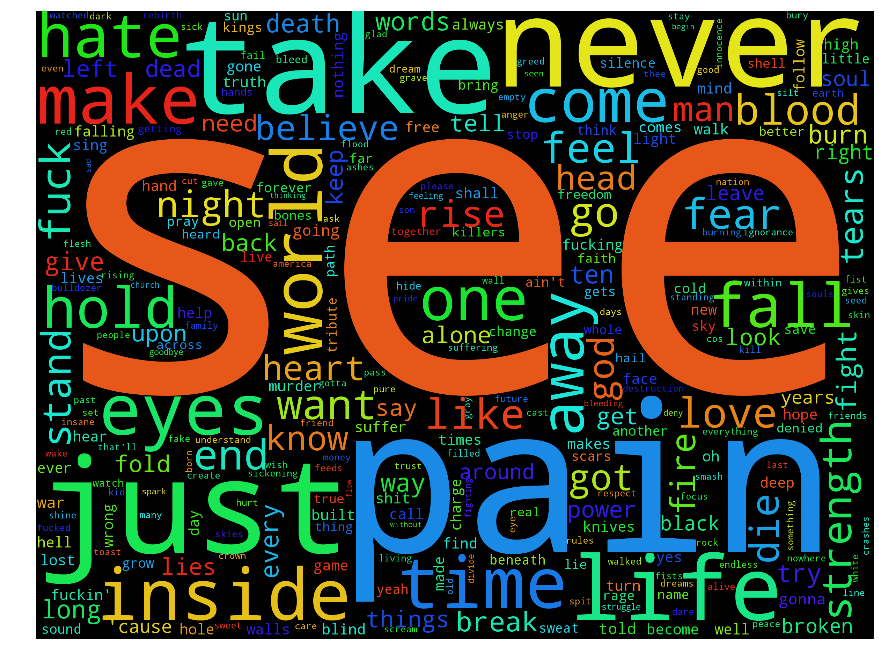
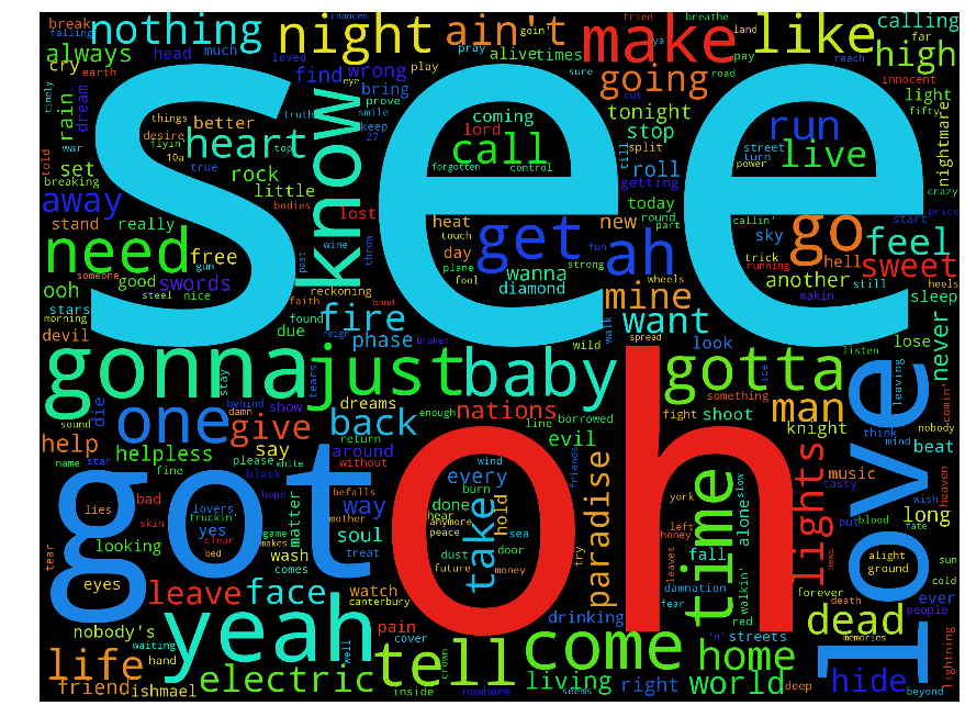
There are some differences, but not a huge amount. The word "see" appears highly in all of them. This is not that surprising: although the bands have slightly different styles, they all play in the same language. If we wanted to emphasis the different usages of language between the band then we need some measure, like "Metalness", but between a number of different sources.
One nice measure of this is the log-likelihood ratio of each word.
The interpretation of the log-likelihood ratio is that we are comparing two hypothesizes: that the word frequencies for each band are drawn from the same distribution or that they are drawn from different distributions. Specifically we assume that the number of occurrences of a target word is binomially distributed (each word in the document either is or isn't the target word). The ratio is given by
Where \(N_{w}\) is number of occurrences of word \(w\) for a specific band, and \(E_{W}\) is the expected occurrence of that word, when considering the distribution for all three bands. \(\bar{N}_{w}\) and \(\bar{E}_{w}\) are the same, but for all words that are not \(w\).
This statistical interpretation models the generation of text as a process of (independently) picking \(n\) words from a predefined distribution multinomial distribution. The log-likelihood ratio then provides a measure for each word how similar the word-distributions are. It is zero when the frequencies of a word are the same for each document, and positive when they are different. It also increases linear with word frequency occurrence.
It should go without saying that such a model for text generation is a huge simplification. Nevertheless, it has the above properties that we would want from a measure of word importance.
Plotting tag clouds of the word sizes proportional to the log likelihood ratio, we get:
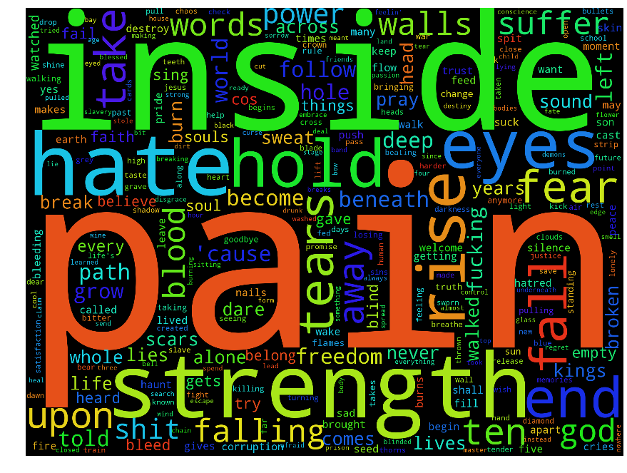
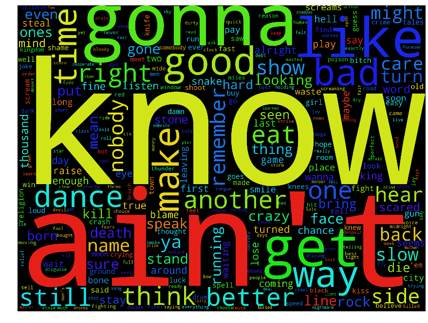
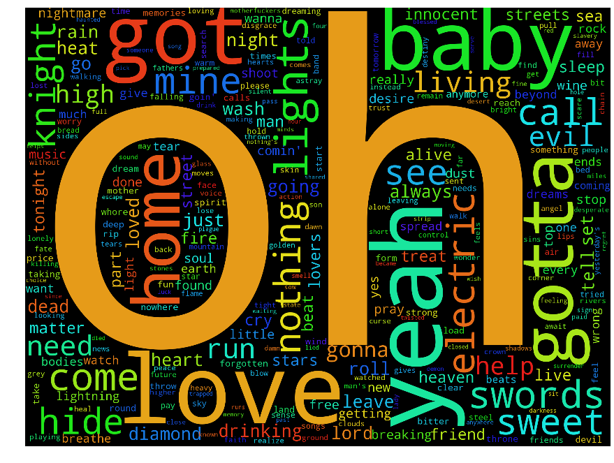
Ordered the same way as before. We seem much more clearly now that one band is about the "pain inside", another "ain't gonna know" and the last is all "oh baby yeah".
VectorHead
Log likelihood provides a measure of the importance of each word to a specific band, but it is not the only one. Another popular measure of word importance is term frequency -Inverse document frequency (TF-IDF). The TF-IDF is a measure of the frequency of word occurrence in a document, weighted by the inverse document frequency: the number of documents in which that word appears. The basic idea is simple, if a word appears in lots of documents, it is probably less important then words that appears only in a few documents. Scikit-learn provides a nice interface to calculate TF-IDF, so I'm going to use it in this section.
We use TF-IDF to compare language use over a number of documents - in this case I am defining a document to be the lyrics to one song. To get a collection of lyrics, I am going to use 15,000 songs by the 119 of some of the more popular artists in our dataset. To keep the dataset manageable we ignore stop words and words that occur in less than 1% of songs, but I do include bi-grams and tri-grams. Also, when splitting words into tokens, I have chosen to keep abbreviations as one word, e.g. "ain't" stays one token, rather then being split or stemmed. This choice was made in an attempt to capture the "style" used by a band, as well as topics.
The result of this vectorization (carried out using sklearn) is that the lyrics of each song is now represented as a vector of 10,000 values.
To get a clearer idea of what is going on here, let's look at a single song: Motorhead's mighty Orgasmatron. Below you can see the full lyrics, with each word coloured depending on it's inverse document frequency importance. Words in black aren't included as they are either too common or too rare, and the IDF score runs from red for low to yellow for high.
Motorhead - Orgasmatron
I am the one, orgasmatron, the outstretched grasping handmy image is of agony, my servants rape the landobsequious and arrogant, clandestine and vaintwo thousand years of misery, of torture in my namehypocrisy made paramount, paranoia the lawmy name is called religion, sadistic, sacred whore .I twist the truth, I rule the world, my crown is called deceitI am the emperor of lies, you grovel at my feetI rob you and I slaughter you, your downfall is my gainand still you play the sycophant and revel in you painand all my promises are lies, all my love is hateI am the politician, and I decide your fateI march before a martyred world, an army for the fightI speak of great heroic days, of victory and mightI hold a banner drenched in blood, I urge you to be bravei lead you to your destiny, I lead you to your graveyour bones will build my palaces, your eyes will stud my crownfor I am mars, the god of war, and I will cut you down .
The first thing to note is that only 79 different words are coloured - this means that the vector describing this song is sparse. The largest 10 values in the TF-IDF vector for this song are, along with their IDF weighting:
| Word | TF-IDF | IDF |
|---|---|---|
| crown | 10.00 | 5.00 |
| called | 9.94 | 4.97 |
| lead | 8.76 | 4.38 |
| decide fate | 7.77 | 7.77 |
| god war | 7.64 | 7.64 |
| palaces | 7.64 | 7.64 |
| two thousand | 7.64 | 7.64 |
| politician | 7.58 | 7.58 |
| arrogant | 7.52 | 7.52 |
| rule world | 7.23 | 7.23 |
Showing that both frequency and IDF contribute to the weighting of a particular word.
DistanceHead
We now have a vector that describes each song - what this allows us to do is in some sense quantify how different two songs are. There are a number of different ways of defining distance in this situation, but a common choice for vectors like this is the cosine distance, as it is insensitive to the total length of the lyric vectors (which in this case would be related to the total number of words in the song).
One major limitation of this approach is that the vectors we are using to represent song lyrics are sparse - even similar songs from the same band are unlikely to have much overlap between them. To get round this, I'm going to stop using vectors on the level of songs, and instead focus on bands. To define a vector for each band, I simply sum together the song vectors for each band.
Using the vector representation of our previous three example bands, we can ask: which are the three most similar bands, which are the three most similar songs to the band and which words are the most important (in terms of having the highest TF-IDF scores) for each band.
| Band | Similar Bands | Most Representative Songs | Most Representative Words |
|---|---|---|---|
| Motorhead | alice cooper, helloween, iron maiden | "Life's A Bitch", "Waiting For The Snake","Desperate For You" | gonna, know, ain't |
| Machinehead | biohazard, metallica, anthrax | "From This Day", "The Blood, The Sweat, The Tears", "Clenching The Fists Of Dissent" | pain, inside, strength |
| Diamondhead | quiet riot, rainbow, wasp | "Victim", "It's Electric", "Wrathchild" | oh, yeah, baby |
What's interesting is that while the most representative songs for each band are mostly their own songs, occasionally other bands songs creep in. For example, "Wrathchild", is an Iron Maiden song, not a Diamondhead song.
Exploring the Lyric Space
Up until now I have been focusing on only three bands because they provided manageable examples, however now that we have a measure of similarity between bands we can open things up. We can start to ask whether the word use in bands lyrics naturally fall into clusters using a technique known as Hierarchical clustering. Essentially we start with each band in its own cluster and one by one, join the clusters together, at each step choosing to merge the two clusters which are closest. The result is a tree-like structure known as a dendrogram, with the branches of similar bands closer together in the tree. Below I've plotted the dendrogram that results from clustering the most popular bands.
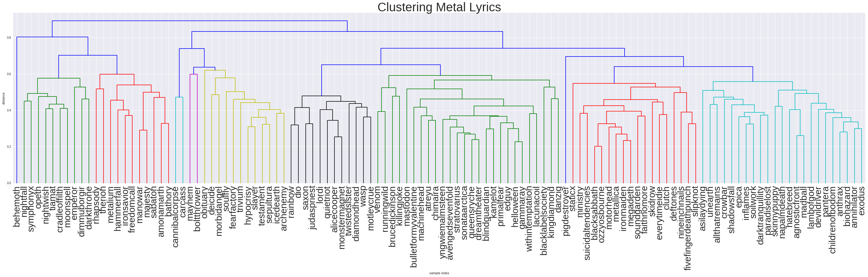
To help explore the diagram above in more depth, I have plotted it using d3 here. By hovering over each node you can get an idea of what the algorithm is doing. Each node represents the cluster at that step, and the tooltip for that cluster shows the most representative bands, songs and words for that node.
In most cases the clustering does a good job of capturing similarity between bands. Ozzy Osborne and Black Sabbath end up close to each other, as do Rainbow and Dio. There is a clear Power Metal grouping, as well as various other small groupings that make vague sense: Madball is next to Agnostic Front; Darkthrone, Dimmu Borgir and Emperor are all close together; Cannabal Corpse and Carcass wallow together in gore.
Exploring the most representative songs for each band we find that certain songs keep appearing: "Six degrees of inner turbulance", Dream theatre and "Narration" by WASP. The reason for this is that these are really long songs. "Six degrees of inner turbulance" clocks in at 45 minutes, long even by dream theatre standards. I'm not even sure "Narration" is a song, but rather the intro to WASPs concept album "The Crimson Idol". This should be taken into account when using interpreting the most representative songs - things can be skewed by length of song, and by other factors I haven't considered here.
Let's recap on what we've done here. By starting with the word frequencies of different bands, we have created a n-dimensional representation of each band and used this to group bands together into similar clusters. With each of these clusters we have tried to explain what is makes it a cluster by looking at representative words, bands and songs.
While we don't have any specific goal in mind with this dataset it is useful to ask: how else might we try and visualise it? This involves reducing our band vectors from an n-dimensional space down to a 2-dimensional space. A common way to do this is with T-SNE. The result is below:
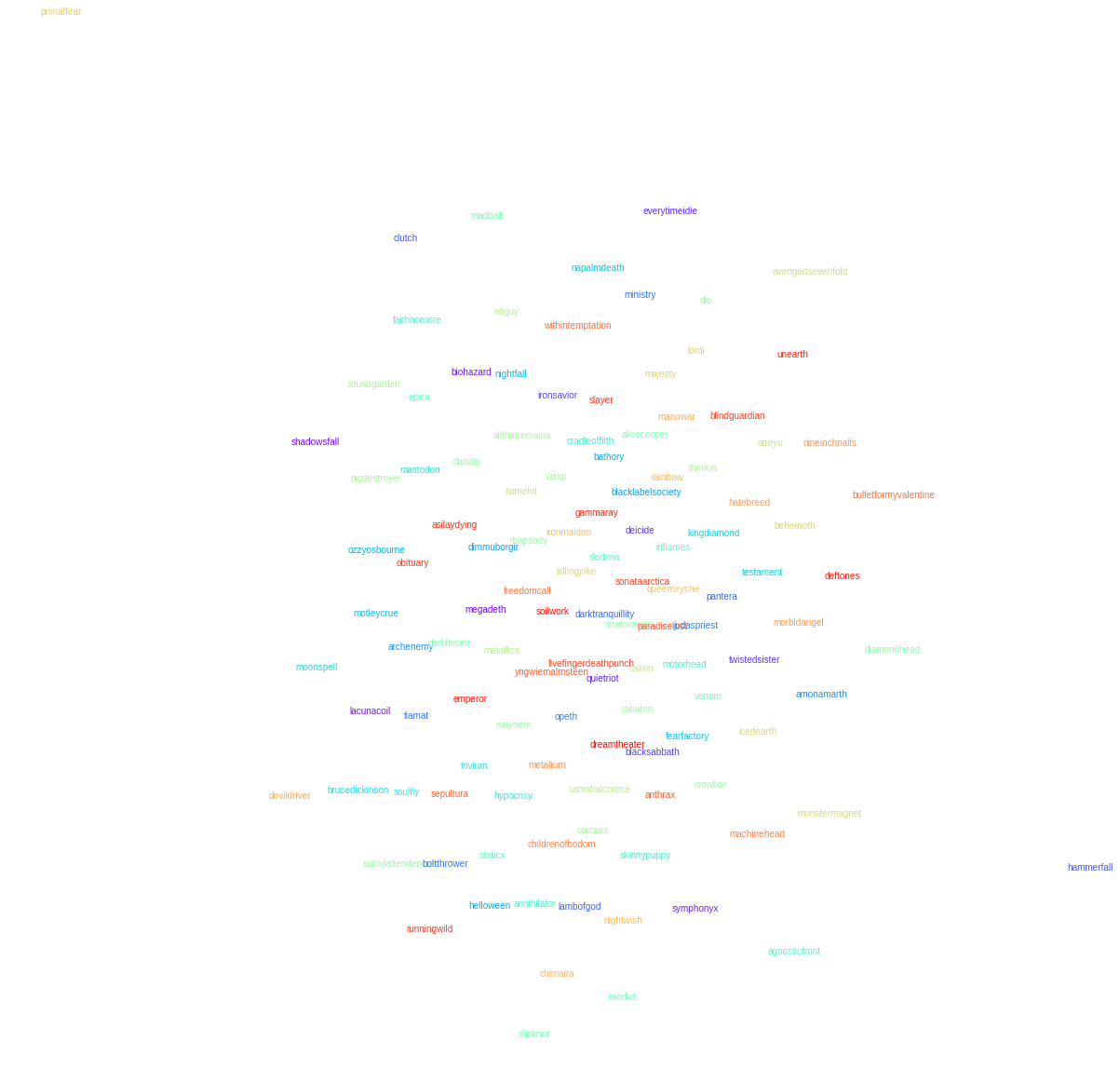
And it's a mess.
T-SNE tried to embed higher dimensional vectors into a lower dimensional space in such a way that if we think of the distances between vectors in the higher dimensional space as Gaussian pairwise probability distributions and the distances between vectors in the lower dimensional space as T-distributed pairwise probability distributions, the embedding tries to minimize the distance between these two distributions for each point.
This suggests why the T-SNE plot above is such a mess. The distances between the band vectors are about the same: somewhere between 0.4 and 0.8. While there is clearly enough structure in these distances to identify clusters, there isn't enough to form a good embedding. There just isn't enough space to embed 120 evenly spaced points in a two dimensional space, and the plot ends up uninformative.
Another way to visualise the band vectors is as a network: we consider each edge as a measure of similarity of the bands. The question is how we choose to connect two bands along an edge. One approach might be to connect two bands if their cosine distance is smaller than a cutoff. The problem with this approach is that we usually end up with tightly connected clusters, mostly disconnected from each other, making visualisation of the space hard.
To get around this, I have used a different measure of similarity: predictability. Consider the following problem: given a description of a song in lyrics space, can we predict which band that song belongs to? This is a standard classification problem, and scikit-learn gives us a whole host of ways to approach this problem. Specifically: I reduced the dimension of the lyric space to 150 dimensions using latent semantic analysis and used a one vs rest logistic regression classifier to make band predictions. Using 10-fold cross validation, the classifier was trained on 90% of the songs (stratified so each band was equally represented in each fold) and then evaluated on the remained 10% of the songs. Band similarity was then measured by the number of times two bands had their songs confused with each other in the test set, averaged over all 10-folds.
Despite classifying a song to one of 120 different bands, the classifier had a precision and recall both around 0.3, with negligible hyper parameter tuning. I tried using other classifiers, such as random forests, and although they obtained higher precision and recall, they exhibited strange behavior. Specifically, when wrong, the random forest classifier, classifier a lot of bands as either Napalm Death or Alice Cooper. I have no idea why, and couldn't explain the results by eyeballing the input features, so I stuck to classifiers that were less "black box".
With this measure of similarity, I can consider two bands connected if they are confused for one another a certain number of times by our classifier and plot the results as the following graphs, produced with graphviz:
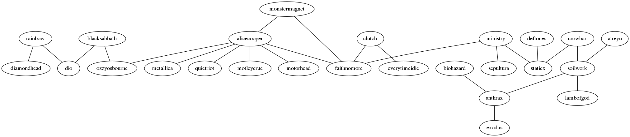
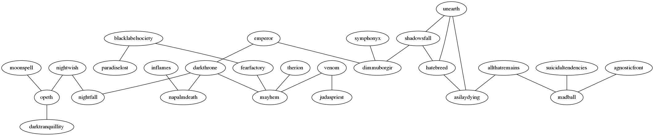
Setting the cutoff at a point where the graph become managably visualisable results in two disconnected subgraphs.
Conclusions
In this post I have looked at using the bag-of-words representation to quantify song lyrics, specifically using metal lyrics as an example. Of course, these methods don't just apply to metal lyrics, we could apply them to any style or genre. It would be interesting to see how far these methods can be taken to identify similar bands and identify genres.
The dataset I have is unlabeled with respect to which genre each band belongs to, but I wouldn't be surprised if the vectors could be used to identify style and even as part of a recommendation engine to find new, similar bands.
Another direction could be to trace out how different styles change over time. If we could link a date to each song, we could potentially see how topics for songs and styles evolve. You might be able to see how bands influence each other. At present I am not aware of anyone looking into this before, but if you have, I'd love to hear about it.
Something I do hope to explore in future blog posts is using the dataset collected for this post to build generative models of text. But that will have to wait for another day (Edit: It's done. You see find the results here). As a taster, here I'll leave you with a few haiku's that I "found" hiding in the metal lyrics:
Burn motherfucker
feel the flame listen to the
whiplash crack your brain
- Pale Rider, Gamma Ray

Freaking out foaming
at the mouth you leave a trail
of dead behind you
- Bite like a Bulldog, Lordi

I part the bloody
hide put my dick right in her
cum is getting thin
- Hand of Doom, Danzig
How was it made
All graphs were produced in python using matplotlib and the seaborn package. The text manipulation was done using sklearn and the nltk.
Comments !